报告函数

本节解释了一些帮助我们创建 Jupyter Notebook 和 Excel 报告的函数,帮助我们快速分析投资组合的属性。
下面的例子创建了一个最佳投资组合,并使用本模块的函数创建了 Jupyter Notebook 和 Excel 报告。
例子
import numpy as np
import pandas as pd
import yfinance as yf
import riskfolio as rp

yf.pdr_override()

# Date range
start = '2016-01-01'
end = '2019-12-30'

# Tickers of assets
tickers = ['JCI', 'TGT', 'CMCSA', 'CPB', 'MO', 'APA', 'MMC', 'JPM',
           'ZION', 'PSA', 'BAX', 'BMY', 'LUV', 'PCAR', 'TXT', 'TMO',
           'DE', 'MSFT', 'HPQ', 'SEE', 'VZ', 'CNP', 'NI', 'T', 'BA']
tickers.sort()

# Downloading the data
data = yf.download(tickers, start = start, end = end)
data = data.loc[:,('Adj Close', slice(None))]
data.columns = tickers
assets = data.pct_change().dropna()

Y = assets

# Creating the Portfolio Object
port = rp.Portfolio(returns=Y)

# To display dataframes values in percentage format
pd.options.display.float_format = '{:.4%}'.format

# Choose the risk measure
rm = 'MV'  # Standard Deviation

# Estimate inputs of the model (historical estimates)
method_mu='hist' # Method to estimate expected returns based on historical data.
method_cov='hist' # Method to estimate covariance matrix based on historical data.

port.assets_stats(method_mu=method_mu, method_cov=method_cov, d=0.94)

# Estimate the portfolio that maximizes the risk adjusted return ratio
w = port.optimization(model='Classic', rm=rm, obj='Sharpe', rf=0.0, l=0, hist=True)
模块函数
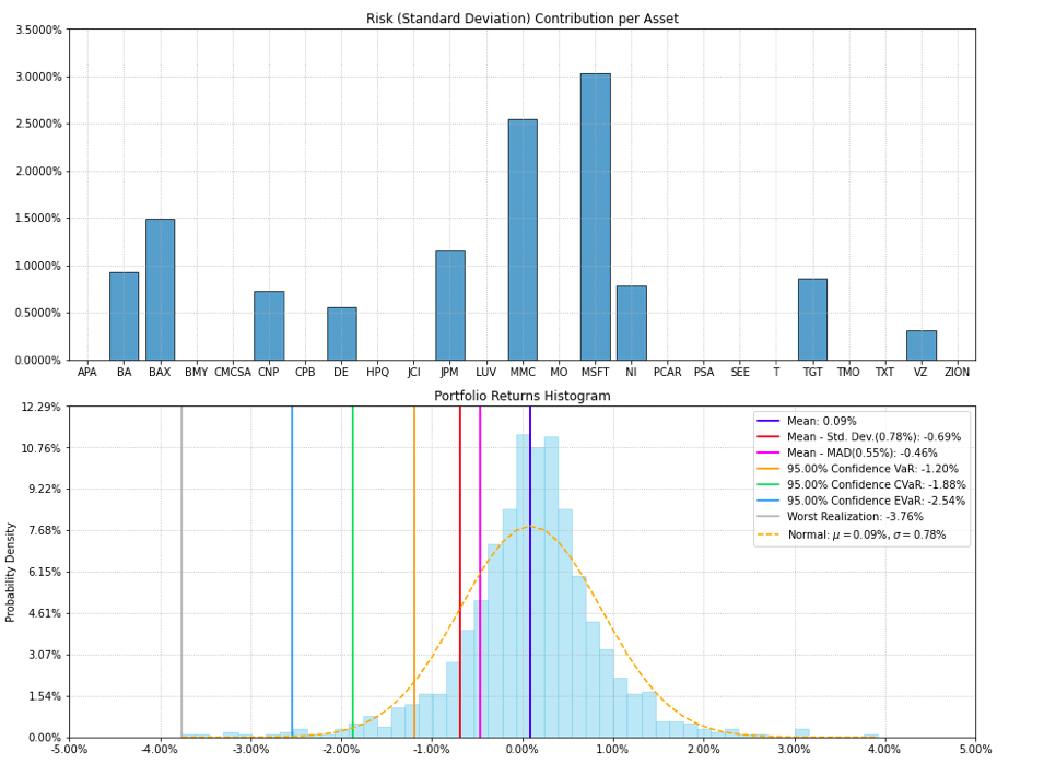
- Reports.jupyter_report(returns, w, rm='MV', rf=0, alpha=0.05, a_sim=100, beta=None, b_sim=None, kappa=0.3, solver=None, percentage=False, erc_line=True, color='tab:blue', erc_linecolor='r', others=0.05, nrow=25, cmap='tab20', height=6, width=14, t_factor=252, ini_days=1, days_per_year=252, bins=50)[源代码]
Create a matplotlib report with useful information to analyze risk and profitability of investment portfolios.
- 参数:
returns (DataFrame) – Assets returns.
w (DataFrame of shape (n_assets, 1)) – Portfolio weights.
rm (str, optional) –
Risk measure used to estimate risk contribution. The default is ‘MV’. Possible values are:
’MV’: Standard Deviation.
’KT’: Square Root Kurtosis.
’MAD’: Mean Absolute Deviation.
’GMD’: Gini Mean Difference.
’MSV’: Semi Standard Deviation.
’SKT’: Square Root Semi Kurtosis.
’FLPM’: First Lower Partial Moment (Omega Ratio).
’SLPM’: Second Lower Partial Moment (Sortino Ratio).
’CVaR’: Conditional Value at Risk.
’TG’: Tail Gini.
’EVaR’: Entropic Value at Risk.
’RLVaR’: Relativistc Value at Risk.
’WR’: Worst Realization (Minimax).
’CVRG’: CVaR range of returns.
’TGRG’: Tail Gini range of returns.
’RG’: Range of returns.
’MDD’: Maximum Drawdown of uncompounded cumulative returns (Calmar Ratio).
’ADD’: Average Drawdown of uncompounded cumulative returns.
’DaR’: Drawdown at Risk of uncompounded cumulative returns.
’CDaR’: Conditional Drawdown at Risk of uncompounded cumulative returns.
’EDaR’: Entropic Drawdown at Risk of uncompounded cumulative returns.
’RLDaR’: Relativistic Drawdown at Risk of uncompounded cumulative returns.
’UCI’: Ulcer Index of uncompounded cumulative returns.
rf (float, optional) – Risk free rate or minimum acceptable return. The default is 0.
alpha (float, optional) – Significance level of VaR, CVaR, Tail Gini, EVaR, RLVaR, CDaR, EDaR and RLDaR. The default is 0.05. The default is 0.05.
a_sim (float, optional) – Number of CVaRs used to approximate Tail Gini of losses. The default is 100.
beta (float, optional) – Significance level of CVaR and Tail Gini of gains. If None it duplicates alpha value. The default is None.
b_sim (float, optional) – Number of CVaRs used to approximate Tail Gini of gains. If None it duplicates a_sim value. The default is None.
kappa (float, optional) – Deformation parameter of RLVaR and RLDaR, must be between 0 and 1. The default is 0.30.
solver (str, optional) – Solver available for CVXPY that supports power cone programming. Used to calculate RLVaR and RLDaR. The default value is None.
percentage (bool, optional) – If risk contribution per asset is expressed as percentage or as a value. The default is False.
erc_line (bool, optional) – If equal risk contribution line is plotted. The default is False.
color (str, optional) – Color used to plot each asset risk contribution. The default is ‘tab:blue’.
erc_linecolor (str, optional) – Color used to plot equal risk contribution line. The default is ‘r’.
others (float, optional) – Percentage of others section. The default is 0.05.
nrow (int, optional) – Number of rows of the legend. The default is 25.
cmap (cmap, optional) – Color scale used to plot each asset weight. The default is ‘tab20’.
height (float, optional) – Average height of charts in the image in inches. The default is 6.
width (float, optional) – Width of the image in inches. The default is 14.
t_factor (float, optional) –
Factor used to annualize expected return and expected risks for risk measures based on returns (not drawdowns). The default is 252.
\[\begin{split}\begin{align} \text{Annualized Return} & = \text{Return} \, \times \, \text{t_factor} \\ \text{Annualized Risk} & = \text{Risk} \, \times \, \sqrt{\text{t_factor}} \end{align}\end{split}\]ini_days (float, optional) – If provided, it is the number of days of compounding for first return. It is used to calculate Compound Annual Growth Rate (CAGR). This value depend on assumptions used in t_factor, for example if data is monthly you can use 21 (252 days per year) or 30 (360 days per year). The default is 1 for daily returns.
days_per_year (float, optional) – Days per year assumption. It is used to calculate Compound Annual Growth Rate (CAGR). Default value is 252 trading days per year.
bins (float, optional) – Number of bins of the histogram. The default is 50.
ax (matplotlib axis of size (6,1), optional) – If provided, plot on this axis. The default is None.
- 抛出:
ValueError – When the value cannot be calculated.
- 返回:
ax – Returns the Axes object with the plot for further tweaking.
- 返回类型:
matplotlib axis
示例
ax = rp.jupyter_report(returns,
                       w,
                       rm='MV',
                       rf=0,
                       alpha=0.05,
                       height=6,
                       width=14,
                       others=0.05,
                       nrow=25)
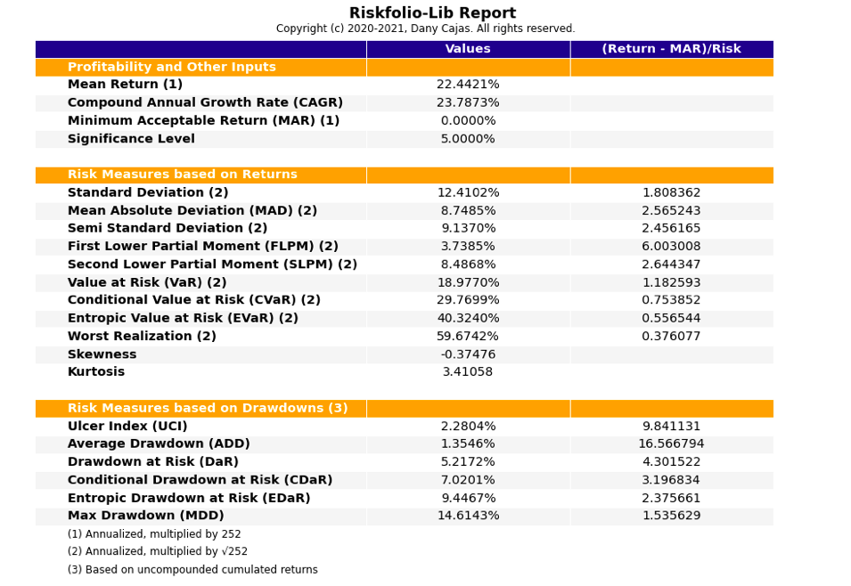


- Reports.excel_report(returns, w, rf=0, alpha=0.05, t_factor=252, ini_days=1, days_per_year=252, name='report')[源代码]
Create an Excel report (with formulas) with useful information to analyze risk and profitability of investment portfolios.
- 参数:
returns (DataFrame) – Assets returns.
w (DataFrame of size (n_assets, n_portfolios)) – Portfolio weights.
rf (float, optional) – Risk free rate or minimum acceptable return. The default is 0.
alpha (float, optional) – Significance level of VaR, CVaR, EVaR, DaR and CDaR. The default is 0.05.
t_factor (float, optional) –
Factor used to annualize expected return and expected risks for risk measures based on returns (not drawdowns). The default is 252.
\[\begin{split}\begin{align} \text{Annualized Return} & = \text{Return} \, \times \, \text{t_factor} \\ \text{Annualized Risk} & = \text{Risk} \, \times \, \sqrt{\text{t_factor}} \end{align}\end{split}\]ini_days (float, optional) – If provided, it is the number of days of compounding for first return. It is used to calculate Compound Annual Growth Rate (CAGR). This value depend on assumptions used in t_factor, for example if data is monthly you can use 21 (252 days per year) or 30 (360 days per year). The default is 1 for daily returns.
days_per_year (float, optional) – Days per year assumption. It is used to calculate Compound Annual Growth Rate (CAGR). Default value is 252 trading days per year.
name (str, optional) – Name or name with path where the Excel report will be saved. If no path is provided the report will be saved in the same path of current file.
- 抛出:
ValueError – When the report cannot be built.
示例
rp.excel_report(returns,
                w,
                rf=0,
                alpha=0.05,
                t_factor=252,
                ini_days=1,
                days_per_year=252,
                name="report")
