约束函数

这个模块有一些功能,可以帮助我们创建任何类型的线性约束条件 与资产或资产类别的权重有关,或与投资组合对特定风险因素的敏感度值有关。 投资组合对某一特定风险因素的敏感性。这些函数将所有 约束的形式 \(Aw\geq B\) 。
此外,该模块还有一个功能,帮助我们为 Black Litterman 模型创建相对和绝对观点。 这种观点可以考虑资产和资产类别之间的关系。这个函数将所有的观点转换为 \(Pw = Q\) 的形式。
模块函数
- ConstraintsFunctions.assets_constraints(constraints, asset_classes)[源代码]
Create the linear constraints matrixes A and B of the constraint \(Aw \geq B\).
- 参数:
constraints (DataFrame of shape (n_constraints, n_fields)) –
Constraints matrix, where n_constraints is the number of constraints and n_fields is the number of fields of constraints matrix, the fields are:
Disabled: (bool) indicates if the constraint is enable.
Type: (str) can be: ‘Assets’, ‘Classes’, ‘All Assets’, ‘Each asset in a class’ and ‘All Classes’.
Set: (str) if Type is ‘Classes’, ‘Each asset in a class’ or ‘All Classes’specified the name of the asset’s classes set.
Position: (str) the name of the asset or asset class of the constraint.
Sign: (str) can be ‘>=’ or ‘<=’.
Weight: (scalar) is the maximum or minimum weight of the absolute constraint.
Type Relative: (str) can be: ‘Assets’ or ‘Classes’.
Relative Set: (str) if Type Relative is ‘Classes’ specified the name of the set of asset classes.
Relative: (str) the name of the asset or asset class of the relative constraint.
Factor: (scalar) is the factor of the relative constraint.
asset_classes (DataFrame of shape (n_assets, n_cols)) – Asset’s classes matrix, where n_assets is the number of assets and n_cols is the number of columns of the matrix where the first column is the asset list and the next columns are the different asset’s classes sets.
- 返回:
A (nd-array) – The matrix A of \(Aw \geq B\).
B (nd-array) – The matrix B of \(Aw \geq B\).
- 抛出:
ValueError when the value cannot be calculated. –
示例
import riskfolio as rp

asset_classes = {'Assets': ['FB', 'GOOGL', 'NTFX', 'BAC', 'WFC', 'TLT', 'SHV'],
                 'Class 1': ['Equity', 'Equity', 'Equity', 'Equity', 'Equity',
                             'Fixed Income', 'Fixed Income'],
                 'Class 2': ['Technology', 'Technology', 'Technology',
                             'Financial', 'Financial', 'Treasury', 'Treasury'],}

asset_classes = pd.DataFrame(asset_classes)
asset_classes = asset_classes.sort_values(by=['Assets'])

constraints = {'Disabled': [False, False, False, False, False, False, False],
               'Type': ['Classes', 'Classes', 'Assets', 'Assets', 'Classes',
                        'All Assets', 'Each asset in a class'],
               'Set': ['Class 1', 'Class 1', '', '', 'Class 2', '', 'Class 1'],
               'Position': ['Equity', 'Fixed Income', 'BAC', 'WFC', 'Financial',
                            '', 'Equity'],
               'Sign': ['<=', '<=', '<=', '<=', '>=', '>=', '>='],
               'Weight': [0.6, 0.5, 0.1, '', '', 0.02, ''],
               'Type Relative': ['', '', '', 'Assets', 'Classes', '', 'Assets'],
               'Relative Set': ['', '', '', '', 'Class 1', '', ''],
               'Relative': ['', '', '', 'FB', 'Fixed Income', '', 'TLT'],
               'Factor': ['', '', '', 1.2, 0.5, '', 0.4]}

constraints = pd.DataFrame(constraints)
The constraint looks like this:
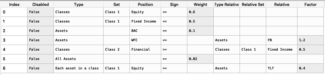
It is easier to construct the constraints in excel and then upload to a dataframe.
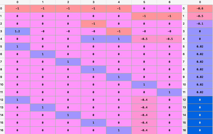
To create the matrixes A and B we use the following command:
A, B = rp.assets_constraints(constraints, asset_classes)
The matrixes A and B looks like this (all constraints were converted to a linear constraint):
- ConstraintsFunctions.factors_constraints(constraints, loadings)[源代码]
Create the factors constraints matrixes C and D of the constraint \(Cw \geq D\).
- 参数:
constraints (DataFrame of shape (n_constraints, n_fields)) –
Constraints matrix, where n_constraints is the number of constraints and n_fields is the number of fields of constraints matrix, the fields are:
Disabled: (bool) indicates if the constraint is enable.
Factor: (str) the name of the factor of the constraint.
Sign: (str) can be ‘>=’ or ‘<=’.
Value: (scalar) is the maximum or minimum value of the factor.
loadings (DataFrame of shape (n_assets, n_features)) – The loadings matrix.
- 返回:
C (nd-array) – The matrix C of \(Cw \geq D\).
D (nd-array) – The matrix D of \(Cw \geq D\).
- 抛出:
ValueError when the value cannot be calculated. –
示例
loadings = {'const': [0.0004, 0.0002, 0.0000, 0.0006, 0.0001, 0.0003, -0.0003],
            'MTUM': [0.1916, 1.0061, 0.8695, 1.9996, 0.0000, 0.0000, 0.0000],
            'QUAL': [0.0000, 2.0129, 1.4301, 0.0000, 0.0000, 0.0000, 0.0000],
            'SIZE': [0.0000, 0.0000, 0.0000, 0.4717, 0.0000, -0.1857, 0.0000],
            'USMV': [-0.7838, -1.6439, -1.0176, -1.4407, 0.0055, 0.5781, 0.0000],
            'VLUE': [1.4772, -0.7590, -0.4090, 0.0000, -0.0054, -0.4844, 0.9435]}

loadings = pd.DataFrame(loadings)

constraints = {'Disabled': [False, False, False],
               'Factor': ['MTUM', 'USMV', 'VLUE'],
               'Sign': ['<=', '<=', '>='],
               'Value': [0.9, -1.2, 0.3],
               'Relative Factor': ['USMV', '', '']}

constraints = pd.DataFrame(constraints)
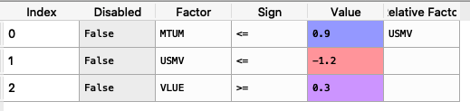
The constraint looks like this:
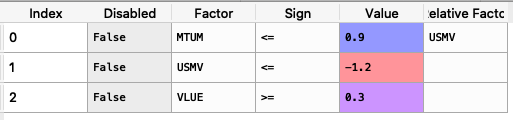
It is easier to construct the constraints in excel and then upload to a dataframe.
To create the matrixes C and D we use the following command:
C, D = rp.factors_constraints(constraints, loadings)
The matrixes C and D looks like this (all constraints were converted to a linear constraint):

- ConstraintsFunctions.assets_views(views, asset_classes)[源代码]
Create the assets views matrixes P and Q of the views \(Pw = Q\).
- 参数:
views (DataFrame of shape (n_views, n_fields)) –
Constraints matrix, where n_views is the number of views and n_fields is the number of fields of views matrix, the fields are:
Disabled: (bool) indicates if the constraint is enable.
Type: (str) can be: ‘Assets’ or ‘Classes’.
Set: (str) if Type is ‘Classes’ specified the name of the set of asset classes.
Position: (str) the name of the asset or asset class of the view.
Sign: (str) can be ‘>=’ or ‘<=’.
Return: (scalar) is the return of the view.
Type Relative: (str) can be: ‘Assets’ or ‘Classes’.
Relative Set: (str) if Type Relative is ‘Classes’ specified the name of the set of asset classes.
Relative: (str) the name of the asset or asset class of the relative view.
asset_classes (DataFrame of shape (n_assets, n_cols)) – Asset’s classes matrix, where n_assets is the number of assets and n_cols is the number of columns of the matrix where the first column is the asset list and the next columns are the different asset’s classes sets.
- 返回:
P (nd-array) – The matrix P that shows the relation among assets in each view.
Q (nd-array) – The matrix Q that shows the expected return of each view.
- 抛出:
ValueError when the value cannot be calculated. –
示例
asset_classes = {'Assets': ['FB', 'GOOGL', 'NTFX', 'BAC', 'WFC', 'TLT', 'SHV'],
                 'Class 1': ['Equity', 'Equity', 'Equity', 'Equity', 'Equity',
                              'Fixed Income', 'Fixed Income'],
                 'Class 2': ['Technology', 'Technology', 'Technology',
                              'Financial', 'Financial', 'Treasury', 'Treasury'],}

asset_classes = pd.DataFrame(asset_classes)
asset_classes = asset_classes.sort_values(by=['Assets'])

views = {'Disabled': [False, False, False, False],
         'Type': ['Assets', 'Classes', 'Classes', 'Assets'],
         'Set': ['', 'Class 2','Class 1', ''],
         'Position': ['WFC', 'Financial', 'Equity', 'FB'],
         'Sign': ['<=', '>=', '>=', '>='],
         'Return': [ 0.3, 0.1, 0.05, 0.03 ],
         'Type Relative': [ 'Assets', 'Classes', 'Assets', ''],
         'Relative Set': [ '', 'Class 1', '', ''],
         'Relative': ['FB', 'Fixed Income', 'TLT', '']}

views = pd.DataFrame(views)
The constraint looks like this:
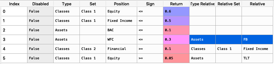
It is easier to construct the constraints in excel and then upload to a dataframe.
To create the matrixes P and Q we use the following command:
P, Q = rp.assets_views(views, asset_classes)
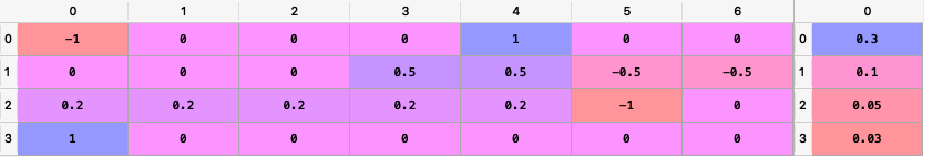
The matrixes P and Q looks like this:
- ConstraintsFunctions.factors_views(views, loadings, const=True)[源代码]
Create the factors constraints matrixes C and D of the constraint \(Cw \geq D\).
- 参数:
constraints (DataFrame of shape (n_constraints, n_fields)) –
Constraints matrix, where n_constraints is the number of constraints and n_fields is the number of fields of constraints matrix, the fields are:
Disabled: (bool) indicates if the constraint is enable.
Factor: (str) the name of the factor of the constraint.
Sign: (str) can be ‘>=’ or ‘<=’.
Value: (scalar) is the maximum or minimum value of the factor.
loadings (DataFrame of shape (n_assets, n_features)) – The loadings matrix.
- 返回:
P (nd-array) – The matrix P that shows the relation among factors in each factor view.
Q (nd-array) – The matrix Q that shows the expected return of each factor view.
- 抛出:
ValueError when the value cannot be calculated. –
示例
loadings = {'const': [0.0004, 0.0002, 0.0000, 0.0006, 0.0001, 0.0003, -0.0003],
            'MTUM': [0.1916, 1.0061, 0.8695, 1.9996, 0.0000, 0.0000, 0.0000],
            'QUAL': [0.0000, 2.0129, 1.4301, 0.0000, 0.0000, 0.0000, 0.0000],
            'SIZE': [0.0000, 0.0000, 0.0000, 0.4717, 0.0000, -0.1857, 0.0000],
            'USMV': [-0.7838, -1.6439, -1.0176, -1.4407, 0.0055, 0.5781, 0.0000],
            'VLUE': [1.4772, -0.7590, -0.4090, 0.0000, -0.0054, -0.4844, 0.9435]}

loadings = pd.DataFrame(loadings)

factorsviews = {'Disabled': [False, False, False],
                'Factor': ['MTUM', 'USMV', 'VLUE'],
                'Sign': ['<=', '<=', '>='],
                'Value': [0.9, -1.2, 0.3],
                'Relative Factor': ['USMV', '', '']}

factorsviews = pd.DataFrame(factorsviews)
The constraint looks like this:
It is easier to construct the constraints in excel and then upload to a dataframe.
To create the matrixes P and Q we use the following command:
P, Q = rp.factors_views(factorsviews, loadings, const=True)
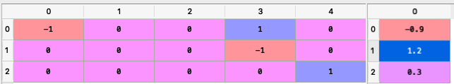
The matrixes P and Q looks like this:
- ConstraintsFunctions.assets_clusters(returns, codependence='pearson', linkage='ward', k=None, max_k=10, bins_info='KN', alpha_tail=0.05, leaf_order=True)[源代码]
Create asset classes based on hierarchical clustering.
- 参数:
returns (DataFrame) – Assets returns.
codependence (str, can be {'pearson', 'spearman', 'abs_pearson', 'abs_spearman', 'distance', 'mutual_info' or 'tail'}) –
The codependence or similarity matrix used to build the distance metric and clusters. The default is ‘pearson’. Possible values are:
’pearson’: pearson correlation matrix. Distance formula: \(D_{i,j} = \sqrt{0.5(1-\rho^{pearson}_{i,j})}\).
’spearman’: spearman correlation matrix. Distance formula: \(D_{i,j} = \sqrt{0.5(1-\rho^{spearman}_{i,j})}\).
’abs_pearson’: absolute value pearson correlation matrix. Distance formula: \(D_{i,j} = \sqrt{(1-|\rho^{pearson}_{i,j}|)}\).
’abs_spearman’: absolute value spearman correlation matrix. Distance formula: \(D_{i,j} = \sqrt{(1-|\rho^{spearman}_{i,j}|)}\).
’distance’: distance correlation matrix. Distance formula \(D_{i,j} = \sqrt{(1-\rho^{distance}_{i,j})}\).
’mutual_info’: mutual information matrix. Distance used is variation information matrix.
’tail’: lower tail dependence index matrix. Dissimilarity formula \(D_{i,j} = -\log{\lambda_{i,j}}\).
linkage (string, optional) –
Linkage method of hierarchical clustering, see linkage for more details. The default is ‘ward’. Possible values are:
’single’.
’complete’.
’average’.
’weighted’.
’centroid’.
’median’.
’ward’.
’DBHT’. Direct Bubble Hierarchical Tree.
k (int, optional) – Number of clusters. This value is took instead of the optimal number of clusters calculated with the two difference gap statistic. The default is None.
max_k (int, optional) – Max number of clusters used by the two difference gap statistic to find the optimal number of clusters. The default is 10.
Number of bins used to calculate variation of information. The default value is ‘KN’. Possible values are:
’KN’: Knuth’s choice method. See more in knuth_bin_width.
’FD’: Freedman–Diaconis’ choice method. See more in freedman_bin_width.
’SC’: Scotts’ choice method. See more in scott_bin_width.
’HGR’: Hacine-Gharbi and Ravier’ choice method.
int: integer value choice by user.
alpha_tail (float, optional) – Significance level for lower tail dependence index. The default is 0.05.
leaf_order (bool, optional) – Indicates if the cluster are ordered so that the distance between successive leaves is minimal. The default is True.
- 返回:
clusters – A dataframe with asset classes based on hierarchical clustering.
- 返回类型:
DataFrame
- 抛出:
ValueError when the value cannot be calculated. –
示例
clusters = rp.assets_clusters(returns, codependence='pearson',
                              linkage='ward', k=None, max_k=10,
                              alpha_tail=0.05, leaf_order=True)
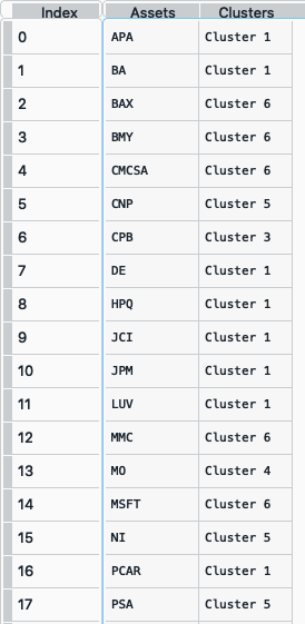
The clusters dataframe looks like this:
- ConstraintsFunctions.hrp_constraints(constraints, asset_classes)[源代码]
Create the upper and lower bounds constraints for hierarchical risk parity model.
- 参数:
constraints (DataFrame of shape (n_constraints, n_fields)) –
Constraints matrix, where n_constraints is the number of constraints and n_fields is the number of fields of constraints matrix, the fields are:
Disabled: (bool) indicates if the constraint is enable.
Type: (str) can be: ‘Assets’, All Assets’ and ‘Each asset in a class’.
Position: (str) the name of the asset or asset class of the constraint.
Sign: (str) can be ‘>=’ or ‘<=’.
Weight: (scalar) is the maximum or minimum weight of the absolute constraint.
asset_classes (DataFrame of shape (n_assets, n_cols)) – Asset’s classes matrix, where n_assets is the number of assets and n_cols is the number of columns of the matrix where the first column is the asset list and the next columns are the different asset’s classes sets.
- 返回:
w_max (pd.Series) – The upper bound of hierarchical risk parity weights constraints.
w_min (pd.Series) – The lower bound of hierarchical risk parity weights constraints.
- 抛出:
ValueError when the value cannot be calculated. –
示例
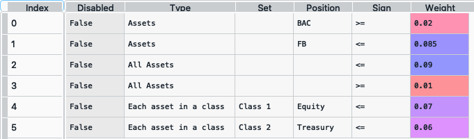
asset_classes = {'Assets': ['FB', 'GOOGL', 'NTFX', 'BAC', 'WFC', 'TLT', 'SHV'],
                 'Class 1': ['Equity', 'Equity', 'Equity', 'Equity', 'Equity',
                             'Fixed Income', 'Fixed Income'],
                 'Class 2': ['Technology', 'Technology', 'Technology',
                             'Financial', 'Financial', 'Treasury', 'Treasury'],}

asset_classes = pd.DataFrame(asset_classes)
asset_classes = asset_classes.sort_values(by=['Assets'])

constraints = {'Disabled': [False, False, False, False, False, False],
               'Type': ['Assets', 'Assets', 'All Assets', 'All Assets',
                        'Each asset in a class', 'Each asset in a class'],
               'Set': ['', '', '', '','Class 1', 'Class 2'],
               'Position': ['BAC', 'FB', '', '', 'Equity', 'Treasury'],
               'Sign': ['>=', '<=', '<=', '>=', '<=', '<='],
               'Weight': [0.02, 0.085, 0.09, 0.01, 0.07, 0.06]}

constraints = pd.DataFrame(constraints)
The constraint looks like this:
It is easier to construct the constraints in excel and then upload to a dataframe.
To create the pd.Series w_max and w_min we use the following command:
w_max, w_min = rp.hrp_constraints(constraints, asset_classes)
The pd.Series w_max and w_min looks like this (all constraints were merged to a single upper bound for each asset):

- ConstraintsFunctions.risk_constraint(asset_classes, kind='vanilla', classes_col=None)[源代码]
Create the risk contribution constraint vector for the risk parity model.
- 参数:
asset_classes (DataFrame of shape (n_assets, n_cols)) – Asset’s classes matrix, where n_assets is the number of assets and n_cols is the number of columns of the matrix where the first column is the asset list and the next columns are the different asset’s classes sets. It is only used when kind value is ‘classes’. The default value is None.
kind (str) –
Kind of risk contribution constraint vector. The default value is ‘vanilla’. Possible values are:
’vanilla’: vector of equal risk contribution per asset.
’classes’: vector of equal risk contribution per class.
classes_col (str or int) – If value is str, it is the column name of the set of classes from asset_classes dataframe. If value is int, it is the column number of the set of classes from asset_classes dataframe. The default value is None.
- 返回:
rb – The risk contribution constraint vector.
- 返回类型:
nd-array
- 抛出:
ValueError when the value cannot be calculated. –
示例
asset_classes = {'Assets': ['FB', 'GOOGL', 'NTFX', 'BAC', 'WFC', 'TLT', 'SHV'],
                 'Class 1': ['Equity', 'Equity', 'Equity', 'Equity', 'Equity',
                              'Fixed Income', 'Fixed Income'],
                 'Class 2': ['Technology', 'Technology', 'Technology',
                              'Financial', 'Financial', 'Treasury', 'Treasury'],}

asset_classes = pd.DataFrame(asset_classes)
asset_classes = asset_classes.sort_values(by=['Assets'])
asset_classes.reset_index(inplace=True, drop=True)

rb = rp.risk_constraint(asset_classes
                        kind='classes',
                        classes_col='Class 1')