结构化预测
在这个\(\newcommand{\reals}{\mathbf{R}}\)\(\newcommand{\ones}{\mathbf{1}}`的例子中,我们使用LLCP对结构化数据拟合回归模型。训练数据集 :math:`D\) 包含 \(N\) 个输入-输出对 \((x, y)\),其中 \(x \in \reals^{n}_{++}\) 是输入,\(y \in \reals^{m}_{++}\) 是输出。每个输出 \(y\) 的条目按升序排序,即 \(y_1 \leq y_2 \leq \cdots \leq y_m\)。
我们的回归模型 \(\phi : \reals^{n}_{++} \to \reals^{m}_{++}\) 接受一个向量 \(x \in \reals^{n}_{++}\) 作为输入,并解决一个LLCP来生成预测 \(\hat y \in \reals^{m}_{++}\)。特别地,LLCP 的解是模型的预测。模型的形式为
这里,最小化是在 \(y \in \reals^{m}_{++}\) 和一个辅助变量 \(z \in \reals^{m}_{++}\) 上进行的,\(\phi(x)\) 是 \(y\) 的最优值,参数为 \(c \in \reals^{m}_{++}\) 和 \(A \in \reals^{m \times n}\)。目标函数中的比率是以元素方式计算的,不等式 \(y \leq z\) 也是如此,\(\ones\) 表示全为1的向量。对于给定的向量 \(x\),这个模型找到一个排序向量 \(\hat y\),其条目接近于 \(x\) 的单项式函数(即 \(z\) 的条目),这是通过分数误差衡量的。
模型在训练集上的训练损失 \(\mathcal{L}(\phi)\) 是均方差损失
我们强调 \(\mathcal{L}(\phi)\) 依赖于 \(c\) 和 \(A\)。在这个例子中,我们拟合LLCP中的参数 \(c\) 和 \(A\),以使训练损失 \(\mathcal{L}(\phi)\) 最小化。**适配中。
** 我们通过在 \(\mathcal L(\phi)\) 上进行迭代的投影梯度下降方法来适配参数。在每次迭代中,我们首先计算训练集中每个输入的预测值 \(\phi(x)\);这需要求解 \(N\) 个LLCPs。接下来,我们评估训练损失 \(\mathcal L(\phi)\)。为了更新参数,我们计算训练损失对参数 \(c\) 和 \(A\) 的梯度 \(\nabla \mathcal L(\phi)\)。这需要通过LLCP的解映射进行微分。我们可以使用CVXPY(或CVXPY Layers)中的 backward 方法高效地计算这个梯度。最后,我们从参数中减去梯度的小倍数。必须注意确保 \(c\) 严格为正;这可以通过将 \(c\) 的条目限制在略高于零的某个小阈值来实现。我们对此方法进行固定次数的迭代。
这个例子在论文 Differentiating through Log-Log Convex Programs 中有描述。
Shane Barratt提出了使用优化层对排序向量进行回归的想法。
要求。 该示例需要PyTorch和CvxpyLayers >= v0.1.3。
from cvxpylayers.torch import CvxpyLayer


import cvxpy as cp
import matplotlib.pyplot as plt
import numpy as np
import torch

torch.set_default_tensor_type(torch.DoubleTensor)
%matplotlib inline
数据生成
n = 20
m = 10

# 训练输入-输出对的数量
N = 100

# 验证对的数量
N_val = 50
torch.random.manual_seed(243)
np.random.seed(243)

normal = torch.distributions.multivariate_normal.MultivariateNormal(torch.zeros(n), torch.eye(n))
lognormal = lambda batch: torch.exp(normal.sample(torch.tensor([batch])))

A_true = torch.randn((m, n)) / 10
c_true = np.abs(torch.randn(m))
def generate_data(num_points, seed):
    torch.random.manual_seed(seed)
    np.random.seed(seed)

    latent = lognormal(num_points)
    noise = lognormal(num_points)
    inputs = noise + latent

    input_cp = op.Parameter(pos=True, shape=(n,))
    prediction = op.multiply(c_true.numpy(), op.gmatmul(A_true.numpy(), input_cp))
    y = op.Variable(pos=True, shape=(m,))
    objective_fn = op.sum(prediction / y + y/prediction)
    constraints = []
    for i in range(m-1):
        constraints += [y[i] <= y[i+1]]
    problem = op.Problem(op.Minimize(objective_fn), constraints)

    outputs = []
    for i in range(num_points):
        input_cp.value = inputs[i, :].numpy()
        problem.solve(op.SCS, gp=True)
        outputs.append(y.value)
    return inputs, torch.stack([torch.tensor(t) for t in outputs])
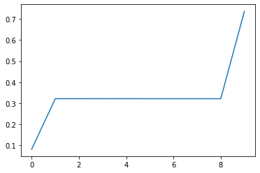
train_inputs, train_outputs = generate_data(N, 243)
plt.plot(train_outputs[0, :].numpy())
[<matplotlib.lines.Line2D at 0x12b367cd0>]
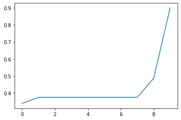
val_inputs, val_outputs = generate_data(N_val, 0)
plt.plot(val_outputs[0, :].numpy())
[<matplotlib.lines.Line2D at 0x12da7e410>]
对每个分量进行单项式拟合
我们将通过对训练数据进行拟合单项式,而不强制施加单调性约束,来初始化我们LLCP模型中的参数。
log_c = cp.Variable(shape=(m,1))
theta = cp.Variable(shape=(n, m))
inputs_np = train_inputs.numpy()
log_outputs_np = np.log(train_outputs.numpy()).T
log_inputs_np = np.log(inputs_np).T
offsets = cp.hstack([log_c]*N)
cp_preds = theta.T @ log_inputs_np + offsets
objective_fn = (1/N) * cp.sum_squares(cp_preds - log_outputs_np)
lstq_problem = cp.Problem(cp.Minimize(objective_fn))
lstq_problem.is_dcp()
True
lstq_problem.solve(verbose=True)
-----------------------------------------------------------------
        OSQP v0.6.0  -  Operator Splitting QP 求解器
           (c) Bartolomeo Stellato, Goran Banjac
     牛津大学 - 斯坦福大学 2019
-----------------------------------------------------------------
问题: 变量 n = 1210,约束 m = 1000
     nnz(P) + nnz(A) = 23000
设置: 线性系统求解器 = qdldl,
     eps_abs = 1.0e-05, eps_rel = 1.0e-05,
     eps_prim_inf = 1.0e-04, eps_dual_inf = 1.0e-04,
     rho = 1.00e-01 (自适应),
     sigma = 1.00e-06, alpha = 1.60, max_iter = 10000
     check_termination: 打开 (间隔 25),
     scaling: 打开, scaled_termination:关闭
     warm start: 打开, polish: 打开, time_limit: 关闭

迭代   目标   主要残差    对偶残差    rho       时间
   1   0.0000e+00   3.30e+00   1.22e+04   1.00e-01   3.06e-03秒
  50   1.0014e-02   1.72e-07   1.64e-07   1.75e-03   7.37e-03秒
plsh   1.0014e-02   1.56e-15   1.17e-14   --------   9.68e-03秒

状态:               求解成功
解的优化:          成功
迭代次数:         50
最优目标:          0.0100
运行时间:        9.68e-03秒
最优rho估计:     8.77e-05
0.010014212812318733
c = torch.exp(torch.tensor(log_c.value)).squeeze()
lstsq_val_preds = []
for i in range(N_val):
    inp = val_inputs[i, :].numpy()
    pred = cp.multiply(c,cp.gmatmul(theta.T.value, inp))
    lstsq_val_preds.append(pred.value)
拟合
A_param = cp.Parameter(shape=(m, n))
c_param = cp.Parameter(pos=True, shape=(m,))
x_slack = cp.Variable(pos=True, shape=(n,))
x_param = cp.Parameter(pos=True, shape=(n,))
y = cp.Variable(pos=True, shape=(m,))

prediction = cp.multiply(c_param, cp.gmatmul(A_param, x_slack))
objective_fn = cp.sum(prediction / y + y / prediction)
constraints = [x_slack == x_param]
for i in range(m-1):
    constraints += [y[i] <= y[i+1]]
problem = cp.Problem(cp.Minimize(objective_fn), constraints)
problem.is_dgp(dpp=True)
True
A_param.value = np.random.randn(m, n)
x_param.value = np.abs(np.random.randn(n))
c_param.value = np.abs(np.random.randn(m))

layer = CvxpyLayer(problem, parameters=[A_param, c_param, x_param], variables=[y], gp=True)
torch.random.manual_seed(1)
A_tch = torch.tensor(theta.T.value)
A_tch.requires_grad_(True)
c_tch = torch.tensor(np.squeeze(np.exp(log_c.value)))
c_tch.requires_grad_(True)
train_losses = []
val_losses = []

lam1 = torch.tensor(1e-1)
lam2 = torch.tensor(1e-1)

opt = torch.optim.SGD([A_tch, c_tch], lr=5e-2)
for epoch in range(10):
    preds = layer(A_tch, c_tch, train_inputs, solver_args={'acceleration_lookback': 0})[0]
    loss = (preds - train_outputs).pow(2).sum(axis=1).mean(axis=0)

    with torch.no_grad():
        val_preds = layer(A_tch, c_tch, val_inputs, solver_args={'acceleration_lookback': 0})[0]
        val_loss = (val_preds - val_outputs).pow(2).sum(axis=1).mean(axis=0)

    print('(epoch {0}) train / val ({1:.4f} / {2:.4f}) '.format(epoch, loss, val_loss))
    train_losses.append(loss.item())
    val_losses.append(val_loss.item())

    opt.zero_grad()
    loss.backward()
    opt.step()
    with torch.no_grad():
        c_tch = torch.max(c_tch, torch.tensor(1e-8))
(历元0)训练 / 验证(0.0018 / 0.0014)
(历元1)训练 / 验证(0.0017 / 0.0014)
(历元2)训练 / 验证(0.0017 / 0.0014)
(历元3)训练 / 验证(0.0017 / 0.0014)
(历元4)训练 / 验证(0.0017 / 0.0014)
(历元5)训练 / 验证(0.0017 / 0.0014)
(历元6)训练 / 验证(0.0016 / 0.0014)
(历元7)训练 / 验证(0.0016 / 0.0014)
(历元8)训练 / 验证(0.0016 / 0.0014)
(历元9)训练 / 验证(0.0016 / 0.0014)
with torch.no_grad():
    train_preds_tch = layer(A_tch, c_tch, train_inputs)[0]
    train_preds = [t.detach().numpy() for t in train_preds_tch]
with torch.no_grad():
    val_preds_tch = layer(A_tch, c_tch, val_inputs)[0]
    val_preds = [t.detach().numpy() for t in val_preds_tch]
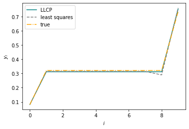
fig = plt.figure()


i = 0
plt.plot(val_preds[i], label='LLCP', color='teal')
plt.plot(lstsq_val_preds[i], label='least squares', linestyle='--', color='gray')
plt.plot(val_outputs[i], label='true', linestyle='-.', color='orange')
w, h = 8, 3.5
plt.xlabel(r'$i$')
plt.ylabel(r'$y_i$')
plt.legend()
plt.show()