全变差修复
灰度图像
灰度图像可以表示为一个 \(m \times n\) 的强度矩阵 \(U^\mathrm{orig}`(通常在值 :math:`0\) 和 \(255\) 之间)。给定值 \(U^\mathrm{orig}_{ij}\),对于 \((i,j) \in \mathcal K\),其中 \(\mathcal K \subset \{1,\ldots, m\} \times \{1, \ldots, n\}\) 是与已知像素值相对应的索引集合。我们的任务是通过猜测丢失的像素值来对图像进行*修复*,即那些索引不在 \(\mathcal K\) 中的像素。重建的图像将由 \(U \in {\bf R}^{m \times n}\) 表示,其中 \(U\) 与已知像素匹配,即对于 \((i,j) \in \mathcal K\),有 \(U_{ij} = U^\mathrm{orig}_{ij}\)。
重建 \(U\) 的步骤是通过最小化 \(U\) 的总变差来实现的,同时要求与已知像素值匹配。我们将使用 \(\ell_2\) 总变差,定义如下:
注意,离散化梯度的范数*不*被平方。
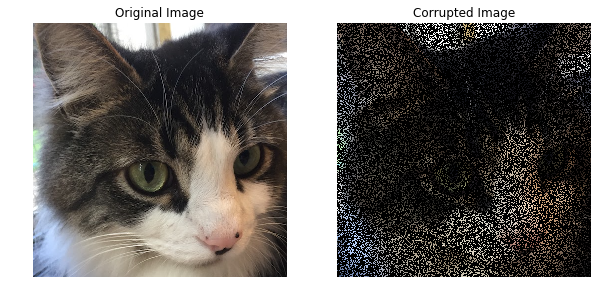
我们加载原始图像和损坏图像,并构建已知矩阵。两个图像如下所示。损坏的图像有缺失的像素被白色覆盖。
import matplotlib.pyplot as plt
import numpy as np

# 加载图像
u_orig = plt.imread("data/loki512.png")
u_corr = plt.imread("data/loki512_corrupted.png")
rows, cols = u_orig.shape

# 如果像素已知,则 known 为 1;
# 如果像素已损坏,则 known 为 0。
known = np.zeros((rows, cols))
for i in range(rows):
    for j in range(cols):
         if u_orig[i, j] == u_corr[i, j]:
            known[i, j] = 1

%matplotlib inline
fig, ax = plt.subplots(1, 2, figsize=(10, 5))
ax[0].imshow(u_orig, cmap='gray')
ax[0].set_title("原始图像")
ax[0].axis('off')
ax[1].imshow(u_corr, cmap='gray');
ax[1].set_title("损坏图像")
ax[1].axis('off');.. image:: tv_inpainting_files/tv_inpainting_2_0.png
总变差修复问题可以很容易地用CVXPY来表示。我们使用了SCS求解器,它能处理比ECOS更大的问题。
# 使用总变差修复恢复原始图像。
import cvxpy as cp


U = cp.Variable(shape=(rows, cols))
obj = cp.Minimize(cp.tv(U))
constraints = [cp.multiply(known, U) == cp.multiply(known, u_corr)]
prob = cp.Problem(obj, constraints)

# 使用SCS求解问题。
prob.solve(verbose=True, solver=cp.SCS)
print("最优目标值: {}".format(obj.value))
----------------------------------------------------------------------------
    SCS v2.0.2 - 分裂锥形求解器
    (c) Brendan O'Donoghue, Stanford University, 2012-2017
----------------------------------------------------------------------------
线性系统: 稀疏的间接方式, A 的非零元素个数 = 1554199, CG公差 ~ 1/iter^(2.00)
eps = 1.00e-05, alpha = 1.50, max_iters = 5000, 标准化 = 1, 缩放 = 1.00
加速回朔 = 20, rho_x = 1.00e-03
变量数目 n = 523265, 约束数目 m = 1045507
锥体: 原始问题的零解 / 对偶问题的自由变量: 262144
    二阶锥变量: 783363, 二阶锥块: 261121
设置时间: 1.23e-01秒
----------------------------------------------------------------------------
 迭代 | 原始残差 | 对偶残差 | 相对间隙 | 原始目标 | 对偶目标 | 卡普/琥珀 | 时间 (秒)
----------------------------------------------------------------------------
     0| 5.19e+00  4.79e+00  1.00e+00 -5.21e+05  1.51e+04  0.00e+00  1.38e+00
   100| 4.46e-03  4.69e-03  3.82e-04  1.10e+04  1.10e+04  3.50e-12  3.95e+01
   200| 3.59e-04  3.83e-04  9.12e-05  1.10e+04  1.10e+04  4.20e-11  7.82e+01
   300| 7.10e-05  6.96e-05  2.77e-05  1.10e+04  1.10e+04  3.75e-11  1.14e+02
   400| 3.30e-05  3.39e-05  2.14e-06  1.10e+04  1.10e+04  6.65e-12  1.47e+02
   500| 2.77e-05  2.85e-05  1.35e-05  1.10e+04  1.10e+04  2.07e-11  1.81e+02
   600| 1.10e-05  1.09e-05  6.45e-06  1.10e+04  1.10e+04  1.48e-11  2.15e+02
   700| 1.00e-05  9.49e-06  1.94e-07  1.10e+04  1.10e+04  2.40e-11  2.48e+02
   720| 9.04e-06  8.24e-06  6.85e-07  1.10e+04  1.10e+04  1.09e-11  2.55e+02
----------------------------------------------------------------------------
状态: 已解决
时间: 解决时间: 2.55e+02秒
    线性系统: 平均CG迭代次数: 9.58, 平均求解时间: 1.41e-01秒
    锥体: 平均投影时间: 3.42e-03秒
    加速: 平均步长时间: 1.71e-01秒
----------------------------------------------------------------------------
误差指标:
dist(s, K) = 2.1720e-04, dist(y, K*) = 3.7180e-04, s'y/|s||y| = -9.9097e-11
原始残差: |Ax + s - b|_2 / (1 + |b|_2) = 9.0439e-06
对偶残差:   |A'y + c|_2 / (1 + |c|_2) = 8.2388e-06
相对间隙:    |c'x + b'y| / (1 + |c'x| + |b'y|) = 6.8544e-07
----------------------------------------------------------------------------
c'x = 11044.2661, -b'y = 11044.2813
============================================================================
最优目标值: 11044.28989542425
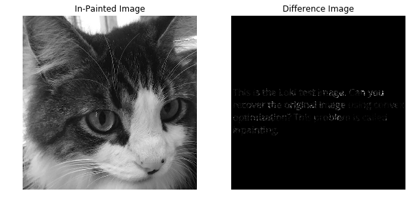
问题求解后,修复后的图像存储在``U.value``中。我们显示修复后的图像和原始图像与修复后图像之间的强度差异。为了更清楚,强度差异放大了10倍。
fig, ax = plt.subplots(1, 2, figsize=(10, 5))
# 显示修复后的图像。
ax[0].imshow(U.value, cmap='gray');
ax[0].set_title("修复后的图像")
ax[0].axis('off')

img_diff = 10*np.abs(u_orig - U.value)
ax[1].imshow(img_diff, cmap='gray');
ax[1].set_title("差异图像")
ax[1].axis('off');
彩色图像
对于彩色图像,修复问题与灰度图像的情况类似。彩色图像可以表示为一个大小为 \(m \times n \times 3\) 的 RGB 值矩阵 \(U^\mathrm{orig}\) (通常取值在 \(0\) 到 \(255\) 之间)。我们已知了一些像素点 \(U^\mathrm{orig}_{ij}\),其中 \((i,j) \in \mathcal K\),其中 \(\mathcal K \subset \{1,\ldots, m\} \times \{1, \ldots, n\}\) 是对应已知像素点的索引集合。每个像素点 \(U^\mathrm{orig}_{ij}\) 是一个大小为 \({\bf R}^3\) 的 RGB 值向量。我们的目标是通过猜测缺失的像素点来修复图像,即索引不属于 \(\mathcal K\) 的像素点。重建图像用 \(U \in {\bf R}^{m \times n \times 3}\) 表示,其中 \(U\) 与已知像素点匹配,即 \(U_{ij} = U^\mathrm{orig}_{ij}\) 对于 \((i,j) \in \mathcal K\)。
我们通过最小化 \(U\) 的总变差来找到重建结果,但要保证匹配已知像素点的值。我们将使用 \(\ell_2\) 总变差,定义为
需要注意的是离散梯度的范数不是平方的。
我们加载原始图像,并通过随机选择保留30%的像素点,丢弃其他像素点,构造了已知矩阵(Known matrix)。下面显示了原始图像和有缺失像素点的损坏图像。损坏图像中的缺失像素点被涂成黑色。
import matplotlib.pyplot as plt
import numpy as np

np.random.seed(1)
# 加载图像。
u_orig = plt.imread("data/loki512color.png")
rows, cols, colors = u_orig.shape

# 如果像素点已知,则 known 为 1,
# 如果像素点受损,则 known 为 0。
# known 矩阵被随机初始化。
known = np.zeros((rows, cols, colors))
for i in range(rows):
    for j in range(cols):
        if np.random.random() > 0.7:
            for k in range(colors):
                known[i, j, k] = 1
u_corr = known * u_orig

# 显示图像。
%matplotlib inline
fig, ax = plt.subplots(1, 2, figsize=(10, 5))
ax[0].imshow(u_orig, cmap='gray');
ax[0].set_title("原始图像")
ax[0].axis('off')
ax[1].imshow(u_corr);
ax[1].set_title("受损图像")
ax[1].axis('off');
We express the total variation color in-painting problem in CVXPY using three matrix variables (one for the red values, one for the blue values, and one for the green values). We use the solver SCS; the solvers ECOS and CVXOPT don’t scale to this large problem.
# Recover the original image using total variation in-painting.
import cvxpy as cp


variables = []
constraints = []
for i in range(colors):
    U = cp.Variable(shape=(rows, cols))
    variables.append(U)
    constraints.append(cp.multiply(known[:, :, i], U) == cp.multiply(known[:, :, i], u_corr[:, :, i]))

prob = cp.Problem(cp.Minimize(cp.tv(*variables)), constraints)
prob.solve(verbose=True, solver=cp.SCS)
print("optimal objective value: {}".format(prob.value))
WARN: A->p (column pointers) not strictly increasing, column 523264 empty
WARN: A->p (column pointers) not strictly increasing, column 785408 empty
WARN: A->p (column pointers) not strictly increasing, column 1047552 empty
----------------------------------------------------------------------------
    SCS v2.0.2 - Splitting Conic Solver
    (c) Brendan O'Donoghue, Stanford University, 2012-2017
----------------------------------------------------------------------------
Lin-sys: sparse-indirect, nnz in A = 3630814, CG tol ~ 1/iter^(2.00)
eps = 1.00e-05, alpha = 1.50, max_iters = 5000, normalize = 1, scale = 1.00
acceleration_lookback = 20, rho_x = 1.00e-03
Variables n = 1047553, constraints m = 2614279
Cones:      primal zero / dual free vars: 786432
    soc vars: 1827847, soc blks: 261121
Setup time: 3.00e-01s
----------------------------------------------------------------------------
 Iter | pri res | dua res | rel gap | pri obj | dua obj | kap/tau | time (s)
----------------------------------------------------------------------------
     0| 1.16e+01  1.18e+01  1.00e+00 -1.02e+06  3.34e+04  1.53e-10  3.81e+00
   100| 2.19e-03  2.32e-03  6.52e-04  1.14e+04  1.15e+04  7.82e-12  1.08e+02
   200| 4.23e-04  3.78e-04  4.97e-05  1.15e+04  1.15e+04  1.34e-11  2.04e+02
   300| 9.58e-05  1.10e-04  5.94e-05  1.15e+04  1.15e+04  1.46e-11  2.96e+02
   400| 4.54e-05  4.57e-05  6.08e-06  1.15e+04  1.15e+04  5.96e-12  3.85e+02
   500| 2.92e-05  3.19e-05  3.42e-06  1.15e+04  1.15e+04  3.37e-11  4.74e+02
   600| 1.77e-05  1.87e-05  1.20e-05  1.15e+04  1.15e+04  3.08e-11  5.60e+02
   700| 1.40e-05  1.43e-05  7.45e-06  1.15e+04  1.15e+04  9.77e-12  6.47e+02
   760| 9.03e-06  9.70e-06  2.43e-06  1.15e+04  1.15e+04  7.02e-12  6.99e+02
----------------------------------------------------------------------------
Status: Solved
Timing: Solve time: 6.99e+02s
    Lin-sys: avg # CG iterations: 11.66, avg solve time: 4.29e-01s
    Cones: avg projection time: 4.72e-03s
    Acceleration: avg step time: 3.94e-01s
----------------------------------------------------------------------------
Error metrics:
dist(s, K) = 1.8769e-05, dist(y, K*) = 1.1246e-04, s'y/|s||y| = 6.2851e-11
primal res: |Ax + s - b|_2 / (1 + |b|_2) = 9.0269e-06
dual res:   |A'y + c|_2 / (1 + |c|_2) = 9.7005e-06
rel gap:    |c'x + b'y| / (1 + |c'x| + |b'y|) = 2.4293e-06
----------------------------------------------------------------------------
c'x = 11465.6528, -b'y = 11465.5971
============================================================================
optimal objective value: 11465.652787130613
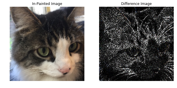
After solving the problem, the RGB values of the in-painted image are stored in the value fields of the three variables. We display the in-painted image and the difference in RGB values at each pixel of the original and in-painted image. Though the in-painted image looks almost identical to the original image, you can see that many of the RGB values differ.
import matplotlib.pyplot as plt
import matplotlib.cm as cm
%matplotlib inline

rec_arr = np.zeros((rows, cols, colors))
for i in range(colors):
    rec_arr[:, :, i] = variables[i].value
rec_arr = np.clip(rec_arr, 0, 1)

fig, ax = plt.subplots(1, 2,figsize=(10, 5))
ax[0].imshow(rec_arr)
ax[0].set_title("修复后的图像")
ax[0].axis('off')

img_diff = np.clip(10 * np.abs(u_orig - rec_arr), 0, 1)
ax[1].imshow(img_diff)
ax[1].set_title("差异图像")
ax[1].axis('off')
(-0.5, 511.5, 511.5, -0.5)