强大的卡尔曼滤波用于车辆跟踪
我们将尝试通过嘈杂的传感器数据准确定位移动车辆的位置。 为此,我们将将车辆状态建模为离散时间线性动态系统。 当传感器噪声被假设为高斯分布时,可以使用标准的**卡尔曼滤波**解决这个问题。 我们将使用**鲁棒卡尔曼滤波**处理非高斯分布的带有离群值的情况,以获得更准确的车辆状态估计。
问题陈述
离散时间线性动态系统由一系列状态向量 \(x_t \in \mathbf{R}^n\) 组成,时间索引为 \(t \in \lbrace 0, \ldots, N-1 \rbrace\), 并且动态方程为
其中 \(w_t \in \mathbf{R}^m\) 是动态系统的输入(例如,车辆上的驱动力), \(y_t \in \mathbf{R}^r\) 是状态测量,\(v_t \in \mathbf{R}^r\) 是噪声, \(A\) 是漂移矩阵,\(B\) 是输入矩阵,\(C\) 是观测矩阵。
给定 \(A\), \(B\), \(C\) 和对于 \(t = 0, \ldots, N-1\) 的 \(y_t\), 目标是估计 \(t = 0, \ldots, N-1\) 的 \(x_t\)。
卡尔曼滤波
卡尔曼滤波通过解决优化问题来估计
where \(\tau\) is a tuning parameter. This problem is actually a least squares problem, and can be solved via linear algebra, without the need for more general convex optimization. Note that since we have no observation \(y_{N}\), \(x_N\) is only constrained via \(x_{N} = Ax_{N-1} + Bw_{N-1}\), which is trivially resolved when \(w_{N-1} = 0\) and \(x_{N} = Ax_{N-1}\). We maintain this vestigial constraint only because it offers a concise problem statement.
This model performs well when \(w_t\) and \(v_t\) are Gaussian. However, the quadratic objective can be influenced by large outliers, which degrades the accuracy of the recovery. To improve estimation in the presence of outliers, we can use robust Kalman filtering.
Robust Kalman filtering
To handle outliers in \(v_t\), robust Kalman filtering replaces the quadratic cost with a Huber cost, which results in the convex optimization problem
where \(\phi_\rho\) is the Huber function
Huber函数惩罚超出半径为:math:(rho) 的估计误差以线性方式,而在标准卡尔曼滤波中,所有的误差都按二次方式进行惩罚。因此,大的误差被惩罚得不那么严厉,使得这个模型对异常值更加鲁棒。
车辆跟踪例子
我们将对具有状态:math:(x_t in mathbf{R}^4)的车辆跟踪问题应用标准和鲁棒的卡尔曼滤波,其中 :math:((x_{t,0}, x_{t,1}))是车辆在两个维度上的位置,:math:((x_{t,2}, x_{t,3}))是车辆的速度。 车辆具有未知的驱动力:math:(w_t),我们观测到车辆位置的噪声测量:math:(y_t in mathbf{R}^2)。
动态矩阵为
其中 \(\gamma\) 是速度阻尼参数。
1D 模型
递归关系源自于单一维度中以下关系。在本小节中, \(x_t, v_t, w_t\) 是车辆的位置、速度和输入驱动力。车辆的加速度为 \(w_t - \gamma v_t\),其中 \(- \gamma v_t\) 是与速度有关的阻尼项,其参数为 \(\gamma\)。
从数值积分得到离散化的动力学方程:
将这些关系扩展到二维,得到动力学矩阵 \(A\) 和 \(B\)。
辅助函数
import matplotlib
import matplotlib.pyplot as plt
import numpy as np

def plot_state(t,actual, estimated=None):
    '''
    plot position, speed, and acceleration in the x and y coordinates for
    the actual data, and optionally for the estimated data
    '''
    trajectories = [actual]
    if estimated is not None:
        trajectories.append(estimated)

    fig, ax = plt.subplots(3, 2, sharex='col', sharey='row', figsize=(8,8))
    for x, w in trajectories:
        ax[0,0].plot(t,x[0,:-1])
        ax[0,1].plot(t,x[1,:-1])
        ax[1,0].plot(t,x[2,:-1])
        ax[1,1].plot(t,x[3,:-1])
        ax[2,0].plot(t,w[0,:])
        ax[2,1].plot(t,w[1,:])

    ax[0,0].set_ylabel('x position')
    ax[1,0].set_ylabel('x velocity')
    ax[2,0].set_ylabel('x input')

    ax[0,1].set_ylabel('y position')
    ax[1,1].set_ylabel('y velocity')
    ax[2,1].set_ylabel('y input')

    ax[0,1].yaxis.tick_right()
    ax[1,1].yaxis.tick_right()
    ax[2,1].yaxis.tick_right()

    ax[0,1].yaxis.set_label_position("right")
    ax[1,1].yaxis.set_label_position("right")
    ax[2,1].yaxis.set_label_position("right")

    ax[2,0].set_xlabel('time')
    ax[2,1].set_xlabel('time')

def plot_positions(traj, labels, axis=None,filename=None):
    '''
    show point clouds for true, observed, and recovered positions
    '''
    matplotlib.rcParams.update({'font.size': 14})
    n = len(traj)

    fig, ax = plt.subplots(1, n, sharex=True, sharey=True,figsize=(12, 5))
    if n == 1:
        ax = [ax]

    for i,x in enumerate(traj):
        ax[i].plot(x[0,:], x[1,:], 'ro', alpha=.1)
        ax[i].set_title(labels[i])
        if axis:
            ax[i].axis(axis)

    if filename:
        fig.savefig(filename, bbox_inches='tight')
Problem Data
We generate the data for the vehicle tracking problem. We’ll have \(N=1000\), \(w_t\) a standard Gaussian, and \(v_t\) a standard Gaussian, except \(20\%\) of the points will be outliers with \(\sigma = 20\).
Below, we set the problem parameters and define the matrices \(A\), \(B\), and \(C\).
n = 1000 # number of timesteps
T = 50 # time will vary from 0 to T with step delt
ts, delt = np.linspace(0,T,n,endpoint=True, retstep=True)
gamma = .05 # damping, 0 is no damping

A = np.zeros((4,4))
B = np.zeros((4,2))
C = np.zeros((2,4))

A[0,0] = 1
A[1,1] = 1
A[0,2] = (1-gamma*delt/2)*delt
A[1,3] = (1-gamma*delt/2)*delt
A[2,2] = 1 - gamma*delt
A[3,3] = 1 - gamma*delt

B[0,0] = delt**2/2
B[1,1] = delt**2/2
B[2,0] = delt
B[3,1] = delt

C[0,0] = 1
C[1,1] = 1
Simulation
We seed \(x_0 = 0\) (starting at the origin with zero velocity) and
simulate the system forward in time. The results are the true vehicle
positions x_true (which we will use to judge our recovery) and the
observed positions y.
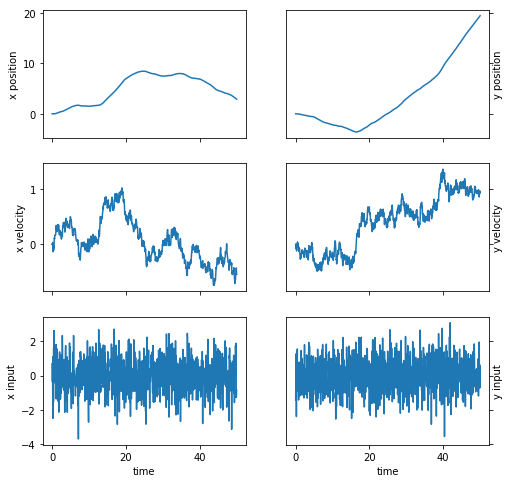
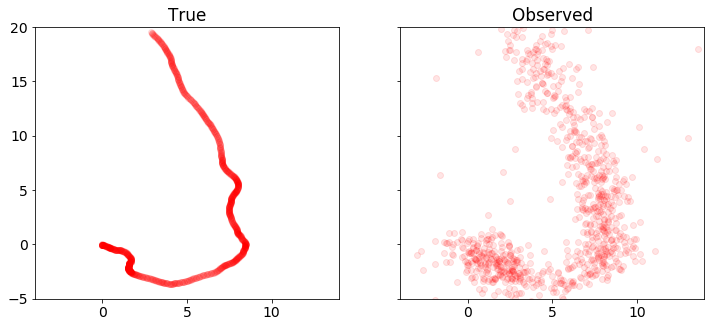
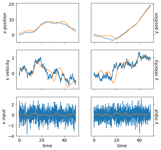
We plot the position, velocity, and system input \(w\) in both dimensions as a function of time. We also plot the sets of true and observed vehicle positions.
sigma = 20
p = .20
np.random.seed(6)

x = np.zeros((4,n+1))
x[:,0] = [0,0,0,0]
y = np.zeros((2,n))

# 生成随机输入和噪声向量
w = np.random.randn(2,n)
v = np.random.randn(2,n)

# 将离群点添加到v中
np.random.seed(0)
inds = np.random.rand(n) <= p
v[:,inds] = sigma*np.random.randn(2,n)[:,inds]

# 模拟系统在时间上的前进
for t in range(n):
    y[:,t] = C.dot(x[:,t]) + v[:,t]
    x[:,t+1] = A.dot(x[:,t]) + B.dot(w[:,t])

x_true = x.copy()
w_true = w.copy()

plot_state(ts,(x_true,w_true))
plot_positions([x_true,y], ['True', 'Observed'],[-4,14,-5,20],'rkf1.pdf')
卡尔曼滤波恢复
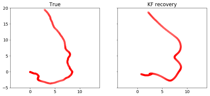
下面的代码使用CVXPY解决标准卡尔曼滤波问题。 我们绘制并比较真实和恢复的车辆状态。注意测量中的离群值会扭曲恢复结果。
%%time
import cvxpy as cp
x = cp.Variable(shape=(4, n+1))
w = cp.Variable(shape=(2, n))
v = cp.Variable(shape=(2, n))
tau = .08
obj = cp.sum_squares(w) + tau*cp.sum_squares(v)
obj = cp.Minimize(obj)
constr = []
for t in range(n):
constr += [ x[:,t+1] == A*x[:,t] + B*w[:,t] ,
y[:,t] == C*x[:,t] + v[:,t] ]
cp.Problem(obj, constr).solve(verbose=True)
x = np.array(x.value)
w = np.array(w.value)
plot_state(ts,(x_true,w_true),(x,w))
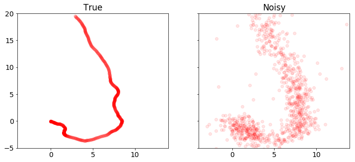
plot_positions([x_true,y], ['True', 'Noisy'], [-4,14,-5,20])
plot_positions([x_true,x], ['True', 'KF recovery'], [-4,14,-5,20], 'rkf2.pdf')
print("optimal objective value: {}".format(obj.value))
-----------------------------------------------------------------
           OSQP v0.4.1  -  操作分裂二次规划求解器
              (c) Bartolomeo Stellato,  Goran Banjac
            牛津大学  -  斯坦福大学 2018
-----------------------------------------------------------------
问题:  变量 n = 8004, 约束 m = 6000
          nnz(P) + nnz(A) = 22000
设置:  线性系统求解器 = qdldl,
          eps_abs = 1.0e-03, eps_rel = 1.0e-03,
          eps_prim_inf = 1.0e-04, eps_dual_inf = 1.0e-04,
          rho = 1.00e-01 (自适应),
          sigma = 1.00e-06, alpha = 1.60, max_iter = 4000
          check_termination: 打开 (间隔 25),
        缩放: 打开, 缩放终止: 关闭
        热启动: 打开, 优化: 打开

迭代  目标函数    主约束残差    对偶约束残差    rho          时间
  1   0.0000e+00   6.14e+01   6.14e+03   1.00e-01   1.28e-02秒
 50   1.1057e+04   3.57e-07   8.27e-08   1.00e-01   3.01e-02秒
plsh  1.1057e+04   7.11e-15   1.24e-14   --------   3.78e-02秒

状态:               解决
优化:               成功
迭代次数:           50
最优目标函数:       11057.3550
运行时间:           3.78e-02秒
最优的rho估计:      7.70e-02

最优目标函数值: 11057.354957764113
CPU时间: 用户 13秒, 系统: 598毫秒, 总计: 13.6秒
墙上时间: 13.8秒

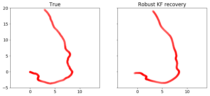
鲁棒卡尔曼滤波恢复
在这里,我们使用CVXPY实现鲁棒卡尔曼滤波。我们可以从下面的图中看到,其恢复效果优于标准的卡尔曼滤波。
%%time
import cvxpy as cp

x = cp.Variable(shape=(4, n+1))
w = cp.Variable(shape=(2, n))
v = cp.Variable(shape=(2, n))

tau = 2
rho = 2

obj = cp.sum_squares(w)
obj += cp.sum([tau*cp.huber(cp.norm(v[:,t]),rho) for t in range(n)])
obj = cp.Minimize(obj)

constr = []
for t in range(n):
    constr += [ x[:,t+1] == A*x[:,t] + B*w[:,t] ,
                y[:,t]   == C*x[:,t] + v[:,t]   ]

cp.Problem(obj, constr).solve(verbose=True)

x = np.array(x.value)
w = np.array(w.value)

plot_state(ts,(x_true,w_true),(x,w))
plot_positions([x_true,y], ['真值', '噪声'], [-4,14,-5,20])
plot_positions([x_true,x], ['真值', '鲁棒卡尔曼滤波恢复'], [-4,14,-5,20],'rkf3.pdf')

print("最优目标值: {}".format(obj.value))
ECOS 2.0.4 - (C) embotech GmbH, 瑞士苏黎世, 2012-15. 网址: www.embotech.com/ECOS

迭代次数  原始松弛系数  对偶松弛系数  间隙    压缩   对偶    开关小型迭代器 范数  步长   有效性   松和    迭代  |   幅
 0  +0.000e+00  -2.923e+02  +7e+05  3e-01  3e-02  1e+00  2e+02    ---    ---    1  1  - |  -  -
 1  +5.090e+02  +4.360e+02  +2e+05  4e-01  1e-02  3e+01  6e+01  0.8051  2e-01   2  1  1 |  0  0
 2  +4.188e+03  +4.134e+03  +2e+05  3e-01  9e-03  3e+01  5e+01  0.4259  6e-01   1  1  1 |  0  0
 3  +9.956e+03  +9.923e+03  +1e+05  3e-01  8e-03  4e+01  4e+01  0.5830  5e-01   1  1  2 |  0  0
 4  +1.881e+04  +1.880e+04  +7e+04  3e-01  5e-03  3e+01  2e+01  0.7189  3e-01   1  1  1 |  0  0
 5  +2.572e+04  +2.572e+04  +4e+04  2e-01  3e-03  2e+01  1e+01  0.5464  3e-01   1  1  1 |  0  0
 6  +2.986e+04  +2.985e+04  +3e+04  2e-01  2e-03  1e+01  6e+00  0.5716  3e-01   2  2  1 |  0  0
 7  +3.262e+04  +3.262e+04  +1e+04  9e-02  1e-03  7e+00  3e+00  0.6007  2e-01   2  2  2 |  0  0
 8  +3.425e+04  +3.425e+04  +8e+03  5e-02  7e-04  5e+00  2e+00  0.5871  3e-01   2  2  2 |  0  0
 9  +3.601e+04  +3.601e+04  +4e+03  3e-02  3e-04  2e+00  9e-01  0.6383  2e-01   2  2  2 |  0  0
10  +3.728e+04  +3.727e+04  +2e+03  1e-02  2e-04  1e+00  5e-01  0.7925  4e-01   2  2  2 |  0  0
11  +3.759e+04  +3.759e+04  +1e+03  1e-02  1e-04  1e+00  3e-01  0.5191  5e-01   2  2  2 |  0  0
12  +3.824e+04  +3.824e+04  +6e+02  6e-03  5e-05  5e-01  2e-01  0.9890  4e-01   2  2  2 |  0  0
13  +3.860e+04  +3.860e+04  +3e+02  3e-03  2e-05  3e-01  7e-02  0.6740  2e-01   2  2  2 |  0  0
14  +3.864e+04  +3.864e+04  +3e+02  3e-03  2e-05  3e-01  7e-02  0.2982  7e-01   2  2  3 |  0  0
15  +3.876e+04  +3.876e+04  +2e+02  2e-03  1e-05  2e-01  4e-02  0.9890  6e-01   2  2  2 |  0  0
16  +3.889e+04  +3.889e+04  +8e+01  1e-03  4e-06  1e-01  2e-02  0.7740  4e-01   3  3  3 |  0  0
17  +3.899e+04  +3.899e+04  +2e+01  4e-04  1e-06  3e-02  6e-03  0.9702  3e-01   3  3  3 |  0  0
18  +3.901e+04  +3.901e+04  +1e+01  4e-04  6e-07  3e-02  4e-03  0.6771  5e-01   4  3  3 |  0  0
19  +3.903e+04  +3.903e+04  +7e+00  2e-04  3e-07  2e-02  2e-03  0.9383  5e-01   3  2  3 |  0  0
20  +3.905e+04  +3.905e+04  +2e+00  1e-04  1e-07  1e-02  6e-04  0.8982  3e-01   4  4  4 |  0  0
21  +3.906e+04  +3.906e+04  +9e-01  5e-05  5e-08  5e-03  2e-04  0.9342  3e-01   3  2  3 |  0  0
22  +3.907e+04  +3.907e+04  +3e-01  4e-05  3e-08  4e-03  8e-05  0.8457  3e-01   5  4  4 |  0  0
23  +3.908e+04  +3.908e+04  +8e-02  1e-05  8e-09  1e-03  2e-05  0.9890  3e-01   3  3  3 |  0  0
24  +3.908e+04  +3.908e+04  +1e-02  2e-06  2e-09  2e-04  3e-06  0.9013  5e-02   3  3  3 |  0  0
25  +3.908e+04  +3.908e+04  +2e-03  4e-07  4e-10  4e-05  5e-07  0.9207  8e-02   3  2  2 |  0  0
26  +3.908e+04  +3.908e+04  +7e-04  2e-07  2e-10  2e-05  2e-07  0.9890  4e-01   2  2  2 |  0  0
27  +3.908e+04  +3.908e+04  +8e-05  3e-08  5e-11  2e-06  2e-08  0.9009  2e-02   2  2  2 |  0  0
28  +3.908e+04  +3.908e+04  +2e-05  1e-08  2e-11  4e-07  5e-09  0.9890  2e-01   2  2  2 |  0  0
29  +3.908e+04  +3.908e+04  +2e-06  3e-09  5e-12  5e-08  5e-10  0.9058  2e-02   2  1  1 |  0  0

OPTIMAL (within feastol=3.1e-09, reltol=5.3e-11, abstol=2.1e-06).
Runtime: 1.129066 seconds.

optimal objective value: 39077.76954636933
CPU times: user 3min 37s, sys: 3.44 s, total: 3min 41s
Wall time: 3min 55s