\(\ell_1\) 趋势滤波

Judon Wilson，在2014年5月28日的基础上进行了衍生改编。改编自Kwangmoo Koh在2007年12月10日的同名CVX示例

主题参考：

• S.-J. Kim, K. Koh, S. Boyd, and D. Gorinevsky，``l_1 Trend Filtering’’、 http://stanford.edu/~boyd/papers/l1_trend_filter.html

介绍

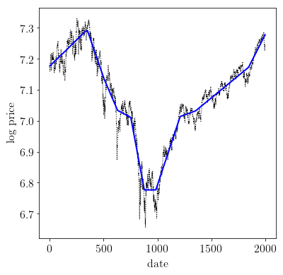
在许多领域中，需要估计时间序列数据中的潜在趋势。l_1 趋势滤波方法可以产生从时间序列``y`` 中得到的分段线性的趋势估计值``x``。

l_1 趋势估计问题可以表述为：

\[\begin{array}{ll} \mbox{最小化} & (1/2)||y-x||_2^2 + \lambda ||Dx||_1, \end{array}\]

其中，变量为 \(x\) ，问题数据为 \(y\) 和 \(\lambda\) ，满足 \(\lambda >0\)。:math:`D`为二阶差分矩阵，行数是….. math:: begin{bmatrix}0 & cdots & 0 & -1 & 2 & -1 & 0 & cdots & 0 end{bmatrix}.

CVXPY 不适用于 \(\ell_1\) 趋势过滤问题。 对于大规模问题，请使用 l1_tf (https://www.stanford.edu/~boyd/l1_tf/)。

制定和解决问题

import numpy as np
import cvxpy as cp
import scipy as scipy
import cvxopt as cvxopt

# 加载时间序列数据：S&P 500 价格的对数。
y = np.loadtxt(open('data/snp500.txt', 'rb'), delimiter=",", skiprows=1)
n = y.size

# 形成二阶差分矩阵。
e = np.ones((1, n))
D = scipy.sparse.spdiags(np.vstack((e, -2*e, e)), range(3), n-2, n)

# 设置正则化参数。
vlambda = 50

# 解决 l1 趋势过滤问题。
x = cp.Variable(shape=n)
obj = cp.Minimize(0.5 * cp.sum_squares(y - x)
                  + vlambda * cp.norm(D*x, 1) )
prob = cp.Problem(obj)

# ECOS 和 SCS 求解器在迭代次数限制之前无法收敛。改用 CVXOPT。
prob.solve(solver=cp.CVXOPT, verbose=True)
print('求解器状态: {}'.format(prob.status))

# 检查错误。
if prob.status != cp.OPTIMAL:
    raise Exception("求解器未收敛！")

print("最优目标值: {}".format(obj.value))

     pcost       dcost       gap    pres   dres   k/t
 0:  0.0000e+00 -1.0000e+00  1e+05  1e-01  4e-02  1e+00
 1:  2.2350e-01  1.5374e-01  8e+03  8e-03  3e-03  7e-02
 2:  1.9086e-01  2.3346e-01  1e+03  1e-03  4e-04  6e-02
 3:  3.9403e-01  4.4110e-01  7e+02  7e-04  3e-04  6e-02
 4:  3.5979e-01  4.1278e-01  3e+02  3e-04  1e-04  6e-02
 5:  6.4154e-01  6.4522e-01  2e+01  2e-05  7e-06  4e-03
 6:  9.0480e-01  9.0710e-01  1e+01  1e-05  4e-06  3e-03
 7:  9.9603e-01  9.9825e-01  1e+01  1e-05  4e-06  2e-03
 8:  1.0529e+00  1.0542e+00  6e+00  6e-06  2e-06  1e-03
 9:  1.1994e+00  1.2004e+00  4e+00  4e-06  2e-06  1e-03
10:  1.2689e+00  1.2693e+00  2e+00  2e-06  6e-07  4e-04
11:  1.3728e+00  1.3729e+00  5e-01  5e-07  2e-07  1e-04
12:  1.3802e+00  1.3803e+00  2e-01  2e-07  9e-08  6e-05
13:  1.3965e+00  1.3965e+00  1e-01  1e-07  4e-08  3e-05
14:  1.3998e+00  1.3998e+00  3e-02  3e-08  1e-08  8e-06
15:  1.3999e+00  1.3999e+00  3e-02  3e-08  1e-08  7e-06
16:  1.4011e+00  1.4011e+00  9e-03  9e-09  3e-09  2e-06
17:  1.4013e+00  1.4013e+00  3e-03  3e-09  1e-09  8e-07
18:  1.4014e+00  1.4014e+00  6e-04  6e-10  3e-10  2e-07
19:  1.4014e+00  1.4014e+00  2e-04  2e-10  7e-11  4e-08
20:  1.4014e+00  1.4017e+00  4e-05  4e-11  2e-08  1e-08
21:  1.4014e+00  1.4015e+00  3e-06  4e-12  8e-08  7e-10
22:  1.4014e+00  1.4013e+00  4e-08  4e-13  2e-08  9e-12
找到最优解。
求解器状态: 最优
最优目标值: 1.4014300716775199

结果图

import matplotlib.pyplot as plt

# 在 ipython 中内联显示图形。
%matplotlib inline

# 图形属性。
plt.rc('text', usetex=True)
plt.rc('font', family='serif')
font = {'weight' : 'normal',
        'size'   : 16}
plt.rc('font', **font)

# 绘制原始信号的估计趋势。
plt.figure(figsize=(6, 6))
plt.plot(np.arange(1,n+1), y, 'k:', linewidth=1.0)
plt.plot(np.arange(1,n+1), np.array(x.value), 'b-', linewidth=2.0)
plt.xlabel('日期')
plt.ylabel('对数价格').. parsed-literal::

Text(0, 0.5, 'log price')