设计给定 \(H(\omega)\) 的一个Chebychev 最佳线性相位(FIR)滤波器
Judson Wilson创作的衍生作品, 5/27/2014。改编自同名CVX示例,作者为Almir Mutapcic, 2/2/2006。
主题参考:
Boyd的 “Filter design” 讲义(EE364)
介绍
该程序设计一个FIR滤波器,给定一个期望的频率响应 \(H_\mbox{des}(\omega)\)。 设计通过最大绝对误差(Chebychev范数)来评判。 这是一个凸问题(在采样之后,可以将其公式化为SOCP),可以写成以下形式:
\[\begin{array}{ll}
\mbox{minimize} & \max |H(\omega) - H_\mbox{des}(\omega)|
\quad \mbox{ for } 0 \le \omega \le \pi,
\end{array}\]
其中变量 \(H\) 是频率响应函数,对应于冲激响应 \(h\)。
初始化问题数据
import numpy as np
import cvxpy as cp

#********************************************************************
# Problem specs.
#********************************************************************
# Number of FIR coefficients (including the zeroth one).
n = 20

# Rule-of-thumb frequency discretization (Cheney's Approx. Theory book).
m = 15*n
w = np.linspace(0,np.pi,m)
#********************************************************************
# Construct the desired filter.
#********************************************************************
# Fractional delay.
D = 8.25                # Delay value.
Hdes = np.exp(-1j*D*w)  # Desired frequency response.

# Gaussian filter with linear phase. (Uncomment lines below for this design.)
#var = 0.05
#Hdes = 1/(np.sqrt(2*np.pi*var)) * np.exp(-np.square(w-np.pi/2)/(2*var))
#Hdes = np.multiply(Hdes, np.exp(-1j*n/2*w))
Solve the minimax (Chebychev) design problem
# A is the matrix used to compute the frequency response
# from a vector of filter coefficients:
#     A[w,:] = [1 exp(-j*w) exp(-j*2*w) ... exp(-j*n*w)]
A = np.exp( -1j * np.kron(w.reshape(-1, 1), np.arange(n)))

# Presently CVXPY does not do complex-valued math, so the
# problem must be formatted into a real-valued representation.

# Split Hdes into a real part, and an imaginary part.
Hdes_r = np.real(Hdes)
Hdes_i = np.imag(Hdes)

# Split A into a real part, and an imaginary part.
A_R = np.real(A)
A_I = np.imag(A)

#
# Optimal Chebyshev filter formulation.
#

# h is the (real) FIR coefficient vector, which we are solving for.
h = cp.Variable(shape=n)
# The objective is:
#     minimize max(|A*h-Hdes|)
# but modified into an equivelent form:
#     minimize max( real(A*h-Hdes)^2 + imag(A*h-Hdes)^2 )
# such that all computation is done in real quantities only.
obj = cp.Minimize(
    cp.max(  cp.square(A_R * h - Hdes_r)     # Real part.
           + cp.square(A_I * h - Hdes_i) ) ) # Imaginary part.

# Solve problem.
prob = cp.Problem(obj)
prob.solve()

# Check if problem was successfully solved.
print('Problem status: {}'.format(prob.status))
if prob.status != cp.OPTIMAL:
    raise Exception('CVXPY Error')
print("final objective value: {}".format(obj.value))
Problem status: optimal
final objective value: 0.4999999999999996
Result plots
import matplotlib.pyplot as plt
# 在 ipython 中内联显示图表。
%matplotlib inline
# 图表属性。
plt.rc('text', usetex=True)
plt.rc('font', family='serif')
font = {'weight' : 'normal',
'size' : 16}
plt.rc('font', **font)
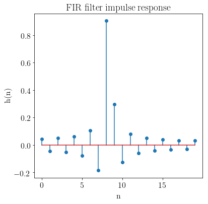
# 绘制 FIR 激励响应。
plt.figure(figsize=(6, 6))
plt.stem(range(n), h.value)
plt.xlabel('n')
plt.ylabel('h(n)')
plt.title('FIR 滤波器激励响应')
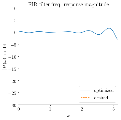
# 绘制频率响应。
H = np.exp(-1j * np.kron(w.reshape(-1, 1), np.arange(n))).dot(h.value)
plt.figure(figsize=(6, 6))
# 幅度
plt.plot(w, 20 * np.log10(np.abs(H)),
label='优化后')
plt.plot(w, 20 * np.log10(np.abs(Hdes)),'--',
label='期望值')
plt.xlabel(r'$\omega$')
plt.ylabel(r'$|H(\omega)|$(分贝)')
plt.title('FIR 滤波器频率响应幅度')
plt.xlim(0, np.pi)
plt.ylim(-30, 10)
plt.legend(loc='lower right')
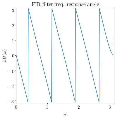
# 相位
plt.figure(figsize=(6, 6))
plt.plot(w, np.angle(H))
plt.xlim(0, np.pi)
plt.ylim(-np.pi, np.pi)
plt.xlabel(r'$\omega$')
plt.ylabel(r'$\angle H(\omega)$')
plt.title('FIR 滤波器频率响应相位')
Text(0.5, 1.0, 'FIR filter freq. response angle')