故障检测

我们将考虑一个基于系统性能传感器测量的问题，即确定系统中已发生的故障。

主题参考

Samar, Sikandar, Dimitry Gorinevsky, and Stephen Boyd. “Likelihood Bounds for Constrained Estimation with Uncertainty.” Decision and Control, 2005 and 2005 European Control Conference. CDC-ECC’05. 44th IEEE Conference on. IEEE, 2005.

问题陈述

每个可能的故障以概率 \(p\) 独立发生。向量 \(x \in \lbrace 0,1 \rbrace^{n}\) 编码了故障的发生情况，其中 \(x_i = 1\) 表示故障 \(i\) 已发生。系统性能由 \(m\) 个传感器测量。传感器输出为

\[\begin{equation} y = Ax + v = \sum_{i=1}^n a_i x_i + v, \end{equation}\]

其中 \(A \in \mathbf{R}^{m \times n}\) 是感知矩阵，其中列 \(a_i\) 是故障 \(i\) 的**故障标识**，而 \(v \in \mathbf{R}^m\) 是一个噪声向量，其中 \(v_j\) 是均值为0、方差为 \(\sigma^2\) 的高斯分布。

目标是根据 \(y`（传感器测量值）猜测 :math:`x`（发生了哪些故障）。我们感兴趣的是 :math:`n > m\) 的情况，也就是说，当我们有更多的潜在错误比测量时。在这种情况下，我们可以期望在向量 \(x\) 稀疏时获得很好的恢复结果。这就是压缩感知的主题。

解决方法

为了识别错误，一种合理的方法是选择 \(x \in \lbrace 0,1 \rbrace^{n}\) 来最小化负对数似然函数

\[\begin{equation} \ell(x) = \frac{1}{2 \sigma^2} \|Ax-y\|_2^2 + \log(1/p-1)\mathbf{1}^T x + c. \end{equation}\]

然而，由于 \(x\) 必须是布尔型的约束条件，这个问题是非凸的且 NP-难的。

为了使这个问题可行，我们可以放宽布尔约束条件，而是约束 \(x_i \in [0,1]\)。

优化问题

\[\begin{split}\begin{array}{ll} \mbox{最小化} & \|Ax-y\|_2^2 + 2 \sigma^2 \log(1/p-1)\mathbf{1}^T x\\ \mbox{满足} & 0 \leq x_i \leq 1, \quad i=1, \ldots n \end{array}凸问题的解称为**放松的ML**估计。\end{split}\]

通过对 \(x\) 的放松的 ML 估计进行四舍五入，将其近似到 0 或 1，我们可以得到一个布尔估计的故障发生情况。

示例

我们将生成一个带有 \(n = 2000\) 个可能故障，\(m = 200\) 个测量和故障概率 \(p = 0.01\) 的示例。我们选择 \(\sigma^2\) 来使得信噪比为 5。也就是说，

\[\begin{equation} \sqrt{\frac{\mathbf{E}\|Ax \|^2_2}{\mathbf{E} \|v\|_2^2}} = 5. \end{equation}\]

import numpy as np
import matplotlib.pyplot as plt

np.random.seed(1)

n = 2000
m = 200
p = 0.01
snr = 5

sigma = np.sqrt(p*n/(snr**2))
A = np.random.randn(m,n)

x_true = (np.random.rand(n) <= p).astype(int)
v = sigma*np.random.randn(m)

y = A.dot(x_true) + v

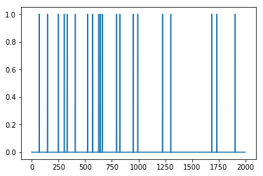
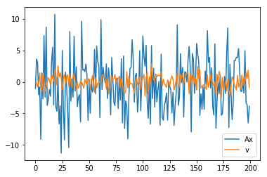
下面，我们展示 \(x\)，\(Ax\) 和噪声 \(v\)。

plt.plot(range(n),x_true)

[<matplotlib.lines.Line2D at 0x11ae42518>]

plt.plot(range(m), A.dot(x_true),range(m),v)
plt.legend(('Ax','v'))

<matplotlib.legend.Legend at 0x11aee9630>

恢复

我们使用CVXPY解决放松的最大似然问题，然后将结果舍入得到布尔解。

##时间
import cvxpy as cp
x = cp.Variable(shape=n)
tau = 2*cp.log(1/p - 1)*sigma**2
obj = cp.Minimize(cp.sum_squares(A*x - y) + tau*cp.sum(x))
const = [0 <= x, x <= 1]
cp.Problem(obj,const).solve(verbose=True)
print("final objective value: {}".format(obj.value))

#放宽的最大似然估计
x_rml = np.array(x.value).flatten()

#舍入解
x_rnd = (x_rml >= .5).astype(int)

ECOS 2.0.4 - (C) embotech GmbH, Zurich Switzerland, 2012-15. Web: www.embotech.com/ECOS

It     pcost       dcost      gap   pres   dres    k/t    mu     step   sigma     IR    |   BT
+7.343e+03  -3.862e+03  +5e+04  5e-01  5e-04  1e+00  1e+01    ---    ---    1  1  - |  -  -
+4.814e+02  -9.580e+02  +8e+03  1e-01  6e-05  2e-01  2e+00  0.8500  1e-02   1  2  2 |  0  0
-2.079e+02  -1.428e+03  +6e+03  1e-01  4e-05  8e-01  2e+00  0.7544  7e-01   2  2  2 |  0  0
-1.321e+02  -1.030e+03  +5e+03  8e-02  3e-05  7e-01  1e+00  0.3122  2e-01   2  2  2 |  0  0
-2.074e+02  -8.580e+02  +4e+03  6e-02  2e-05  6e-01  9e-01  0.7839  7e-01   2  2  2 |  0  0
-1.121e+02  -6.072e+02  +3e+03  5e-02  1e-05  5e-01  7e-01  0.3859  4e-01   2  3  3 |  0  0
-4.898e+01  -4.060e+02  +2e+03  3e-02  8e-06  3e-01  5e-01  0.5780  5e-01   2  2  2 |  0  0
+7.778e+01  -5.711e+01  +8e+02  1e-02  3e-06  1e-01  2e-01  0.9890  4e-01   2  3  2 |  0  0
+1.307e+02  +6.143e+01  +4e+02  6e-03  1e-06  6e-02  1e-01  0.5528  1e-01   3  3  3 |  0  0
+1.607e+02  +1.286e+02  +2e+02  3e-03  4e-07  3e-02  5e-02  0.8303  3e-01   3  3  3 |  0  0
+1.741e+02  +1.557e+02  +1e+02  2e-03  2e-07  2e-02  3e-02  0.6242  3e-01   3  3  3 |  0  0
+1.834e+02  +1.749e+02  +5e+01  8e-04  9e-08  8e-03  1e-02  0.8043  3e-01   3  3  3 |  0  0
+1.888e+02  +1.861e+02  +2e+01  3e-04  3e-08  2e-03  4e-03  0.9175  3e-01   3  3  2 |  0  0
+1.909e+02  +1.902e+02  +4e+00  7e-05  7e-09  6e-04  1e-03  0.8198  1e-01   3  3  3 |  0  0
+1.914e+02  +1.912e+02  +1e+00  2e-05  2e-09  2e-04  3e-04  0.8581  2e-01   3  2  3 |  0  0
+1.916e+02  +1.916e+02  +1e-01  2e-06  3e-10  2e-05  4e-05  0.9004  3e-02   3  3  3 |  0  0
+1.916e+02  +1.916e+02  +4e-02  7e-07  8e-11  7e-06  1e-05  0.8174  1e-01   3  3  3 |  0  0
+1.916e+02  +1.916e+02  +8e-03  1e-07  1e-11  1e-06  2e-06  0.8917  9e-02   3  2  2 |  0  0
+1.916e+02  +1.916e+02  +2e-03  4e-08  4e-12  4e-07  5e-07  0.8588  2e-01   3  3  3 |  0  0
+1.916e+02  +1.916e+02  +2e-04  3e-09  3e-13  3e-08  5e-08  0.9309  2e-02   3  2  2 |  0  0
+1.916e+02  +1.916e+02  +2e-05  4e-10  4e-14  4e-09  6e-09  0.8768  1e-02   4  2  2 |  0  0
+1.916e+02  +1.916e+02  +4e-06  6e-11  6e-15  6e-10  9e-10  0.9089  6e-02   4  2  2 |  0  0
+1.916e+02  +1.916e+02  +1e-06  2e-11  2e-15  2e-10  2e-10  0.8362  1e-01   2  1  1 |  0  0

OPTIMAL (within feastol=1.8e-11, reltol=5.1e-09, abstol=9.8e-07).
Runtime: 6.538894 seconds.

final objective value: 191.6347201927456
CPU times: user 6.51 s, sys: 291 ms, total: 6.8 s
Wall time: 7.5 s

Evaluation

我们定义了一个计算估计误差的函数和一个用于绘制数学公式“x”、松弛最大似然估计和四舍五入解的函数。

import matplotlib

def errors(x_true, x, threshold=.5):
    '''返回估计误差。

    返回真实的故障数量、误报数量和漏报数量。
    '''
    n = len(x_true)
    k = sum(x_true)
    false_pos = sum(np.logical_and(x_true < threshold, x >= threshold))
    false_neg = sum(np.logical_and(x_true >= threshold, x < threshold))
    return (k, false_pos, false_neg)

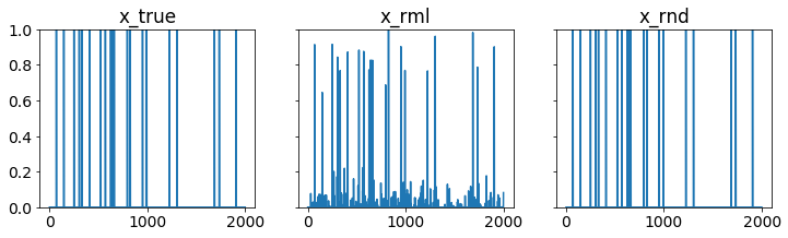
def plotXs(x_true, x_rml, x_rnd, filename=None):
    '''绘制真实、松弛最大似然估计和四舍五入解。'''
    matplotlib.rcParams.update({'font.size': 14})
    xs = [x_true, x_rml, x_rnd]
    titles = ['x_true', 'x_rml', 'x_rnd']

    n = len(x_true)
    k = sum(x_true)

    fig, ax = plt.subplots(1, 3, sharex=True, sharey=True, figsize=(12, 3))

    for i,x in enumerate(xs):
            ax[i].plot(range(n), x)
            ax[i].set_title(titles[i])
            ax[i].set_ylim([0,1])

    if filename:
        fig.savefig(filename, bbox_inches='tight')

    return errors(x_true, x_rml,.5)

我们可以看到，在20个实际故障中，四舍五入解完美恢复，没有漏报和误报。

plotXs(x_true, x_rml, x_rnd, 'fault.pdf')

(20, 0, 0)