时钟网格的尺寸化
原作者:Lieven Vanderberghe。由 Argyris Zymnis 改编为 CVX,日期:2005 年 12 月 4 日。由 Michael Grant 修改,日期:2006 年 3 月 8 日。由 Judson Wilson 改编为 CVXPY,进行了美化修改,日期:2014 年 5 月 26 日。
主题参考:
第 4 节,L. Vandenberghe,S. Boyd,A. El Gamal,《非树形电路的最佳导线和晶体管尺寸化》
引言
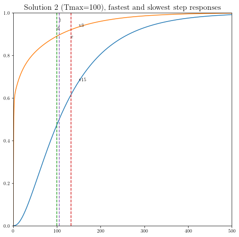
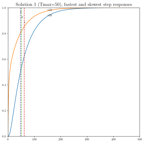
我们考虑尺寸化时钟网格的问题,以使得在主导时间常数的约束下,总耗散功率最小化。网格中的节点数是每行或每列的 \(N`(因此总共为 :math:`n=(N+1)^2\))。我们将导线分成宽度为 \(x_i`(:math:`i = 1,\dots,m\))的 m 个段,这些宽度受到约束 \(0 \le x_i \le W_{\mbox{max}}\)。我们使用每个导线段的 pi 模型,其电容为 \(\beta_i x_i\),电导为 \(\alpha_i x_i\)。定义 \(C(x) = C_0+x_1 C_1 + x_2 C_ 2 + \cdots + x_m C_m\),我们有耗散功率等于 \(\mathbf{1}^T C(x) \mathbf{1}\)。因此,为了在宽度和主导时间常数约束下最小化耗散功率,我们求解 SDP 问题
\[\begin{split}\begin{array}{ll}
\mbox{minimize} & \mathbf{1}^T C(x) \mathbf{1} \\
\mbox{subject to} & T_{\mbox{max}} G(x) - C(x) \succeq 0 \\
& 0 \le x_i \le W_{\mbox{max}}.
\end{array}\end{split}\]
导入和设置包
import cvxpy as cp
import numpy as np
import scipy as scipy
import matplotlib.pyplot as plt

# 在ipython中内联显示绘图。
%matplotlib inline

# 绘图属性。
plt.rc('text', usetex=True)
plt.rc('font', family='serif')
font = {'weight' : 'normal',
        'size'   : 16}
plt.rc('font', **font)
辅助函数
# 计算线性系统的阶跃响应。
def simple_step(A, B, DT, N):
    n  = A.shape[0]
    Ad = scipy.linalg.expm((A * DT))
    Bd = (Ad - np.eye(n)).dot(B)
    Bd = np.linalg.solve(A, Bd)
    X  = np.zeros((n, N))
    for k in range(1, N):
        X[:, k] = Ad.dot(X[:, k-1]) + Bd;
    return X
生成问题数据
#
# 电路参数。
#
dim=4# 网格大小为 dim x dim(假设 dim 是偶数)。
# 节点数。
n=(dim+1)**2
# 导线数。
m=2*dim*(dim+1)
# 0 ... dim(dim+1)-1 是水平段
# (以行优先编号);
# dim(dim+1) ... 2*dim(dim+1)-1 是垂直段
# (以列优先编号)
beta = 0.5
# 每个段的电容是两倍的 beta 倍 xi。
alpha = 1
# 每个段的电导是 alpha 倍 xi。
G0 = 1
C0 = np.array([ ( 10, 2, 7, 5, 3),
( 8, 3, 9, 5, 5),
( 1, 8, 4, 9, 3),
( 7, 3, 6, 8, 2),
( 5, 2, 1, 9, 10) ])
# x 的上限。
wmax = 1
#
# 构建电容和电导矩阵。
#
CC = np.zeros((dim+1, dim+1, dim+1, dim+1, m+1))
GG = np.zeros((dim+1, dim+1, dim+1, dim+1, m+1))
# 常数项。
# - 以 fortran 顺序重塑的原因是为了与 MATLAB 代码中的原始版本相匹配。
CC[:, :, :, :, 0] = np.diag(C0.flatten(order='F')).reshape(dim+1, dim+1,
dim+1, dim+1, order='F').copy()
zo13 = np.zeros((2, 1, 2, 1))
zo13[:,0,:,0] = np.array([(1, 0), (0, 1)])
zo24 = np.zeros((1, 2, 1, 2))
zo24[0,:,0,:] = zo13[:, 0, :, 0]
pn13 = np.zeros((2, 1, 2, 1))
pn13[:,0,:,0] = np.array([[1, -1], [-1, 1]])
pn24 = np.zeros((1, 2, 1, 2))
pn24[0, :, 0, :] = pn13[:, 0, :, 0]
for i in range(dim+1):
# 源电导。
# 第一个驱动器位于第一行的中间。
GG[int(dim/2), i, int(dim/2), i, 0] = G0
for j in range(dim):
# 水平段。
node = 1 + j + i * dim
CC[j:j+2, i, j:j+2, i, node] = beta * zo13[:, 0, :, 0]
GG[j:j+2, i, j:j+2, i, node] = alpha * pn13[:, 0, :, 0]
# 垂直段。
node = node + dim * ( dim + 1 )
CC[i, j:j+2, i, j:j+2, node] = beta * zo24[0, :, 0, :]
GG[i, j:j+2, i, j:j+2, node] = alpha * pn24[0, :, 0, :]
# 重塑便于使用。
CC = CC.reshape((n*n, m+1), order='F').copy()
GG = GG.reshape((n*n, m+1), order='F').copy()
#
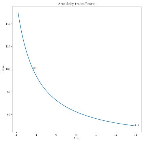
# 计算折衷曲线上的点和三个样本点。
#
npts = 50
delays = np.linspace(50, 150, npts)
xdelays = [50, 100]
xnpts = len(xdelays)
areas = np.zeros(npts)
xareas = dict()
求解问题并显示结果
# 遍历所有点,并重新访问特定点
for i in range(npts + xnpts):
    # 第一次遍历,只收集所有案例的最小数据。
    if i < npts:
        delay = delays[i]
        print( ('Point {} of {} on the tradeoff curve ' \
              + '(Tmax = {})').format(i+1, npts, delay))
    # 第二次遍历,收集特定案例的更多数据,并进行绘图(稍后)。
    else:
        xi = i - npts
        delay = xdelays[xi]
        print( ('Particular solution {} of {} ' \
              + '(Tmax = {})').format(xi+1, xnpts, delay))

    #
    # 构建和求解凸模型。
    #

    # 变量。
    xt = cp.Variable(shape=(m+1)) # 元素 1 的 xt == 1。
    G = cp.Variable((n,n), symmetric=True)  # 对称约束。
    C = cp.Variable((n,n), symmetric=True)  # 对称约束。

    # 目标。
    obj = cp.Minimize(cp.sum(C))

    # 约束。
    constraints = [ xt[0] == 1,
                    G == G.T,
                    C == C.T,
                    G == cp.reshape(GG*xt, (n,n)),
                    C == cp.reshape(CC*xt, (n,n)),
                    delay * G - C == cp.Variable(shape=(n,n), PSD=True),
                    0 <= xt[1:],
                    xt[1:] <= wmax,
                  ]

    # Solve problem (use CVXOPT instead of SCS to match original results;
    # cvxopt produces lower objective values as well, but is much slower)
    prob = cp.Problem(obj, constraints)
    try:
        prob.solve(solver=cp.CVXOPT)
    except cp.SolverError:
        print("CVXOPT failed, trying robust KKT")
        prob.solve(solver=cp.CVXOPT, kktsolver='robust')

    if prob.status not in [cp.OPTIMAL, cp.OPTIMAL_INACCURATE]:
        raise Exception('CVXPY Error')

    # Chop off the first element of x, which is
    # constrainted to be 1
    x = xt.value[1:]

    # First pass, only gather minimal data from all cases.
    if i < npts:
        areas[i] = sum(x)
    # Second pass, gather more data for specific cases,
    # and make plots.
    else:
        xareas[xi] = sum(x)

        #
        # Print display sizes.
        #

        print('Solution {}:'.format(xi+1))
        print('Vertical segments:')
        print(x[0:dim*(dim+1)].reshape(dim, dim+1, order='F').copy())
        print('Horizontal segments:')
        print(x[dim*(dim+1):].reshape(dim, dim+1, order='F').copy())

        #
        # Determine and plot the step responses.
        #

        A = -np.linalg.inv(C.value).dot(G.value)
        B = -A.dot(np.ones(n))
        T = np.linspace(0, 500, 2000)
        Y = simple_step(A, B, T[1], len(T))
        indmax = -1
        indmin = np.inf
        for j in range(Y.shape[0]):
            inds = np.amin(np.nonzero(Y[j, :] >= 0.5)[0])
            if ( inds > indmax ):
                indmax = inds
                jmax = j
            if ( inds < indmin ):
                indmin = inds
                jmin = j

        tthres = T[indmax]
        GinvC  = np.linalg.solve(G.value, C.value)
        tdom   = max(np.linalg.eig(GinvC)[0])
        elmore = np.amax(np.sum(GinvC.T, 0))
        plt.figure(figsize=(8, 8))
        plt.plot( T, np.asarray(Y[jmax,:]).flatten(), '-',
                  T, np.asarray(Y[jmin,:]).flatten() )
        plt.plot( tdom   * np.array([1, 1]), [0, 1], '--',
                  elmore * np.array([1, 1]), [0, 1], '--',
                  tthres * np.array([1, 1]), [0, 1], '--' )
        plt.xlim([0, 500])
        plt.ylim([0, 1])
        plt.text(tdom, 0.92, 'd')
        plt.text(elmore, 0.88, 'e')
        plt.text(tthres, 0.96, 't')
        plt.text( T[600], Y[jmax, 600], 'v{}'.format(jmax+1))
        plt.text( T[600], Y[jmin, 600], 'v{}'.format(jmin+1))
        plt.title(('Solution {} (Tmax={}), fastest ' \
                    + 'and slowest step responses').format(xi+1, delay), fontsize=16)
        plt.show()

#
# Plot the tradeoff curve.
#

plt.figure(figsize=(8, 8))
ind = np.isfinite(areas)
plt.plot(areas[ind], delays[ind])
plt.xlabel('Area')
plt.ylabel('Tdom')
plt.title('Area-delay tradeoff curve')
# Label the specific cases.
for k in range(xnpts):
    plt.text(xareas[k], xdelays[k], '({})'.format(k+1))
plt.show()
在权衡曲线上的第1点(Tmax = 50.0)
CVXOPT失败,尝试鲁棒KKT
在权衡曲线上的第2点(Tmax = 52.04081632653061)
在权衡曲线上的第3点(Tmax = 54.08163265306123)
在权衡曲线上的第4点(Tmax = 56.12244897959184)
在权衡曲线上的第5点(Tmax = 58.16326530612245)
在权衡曲线上的第6点(Tmax = 60.20408163265306)
在权衡曲线上的第7点(Tmax = 62.244897959183675)
在权衡曲线上的第8点(Tmax = 64.28571428571429)
在权衡曲线上的第9点(Tmax = 66.3265306122449)
在权衡曲线上的第10点(Tmax = 68.36734693877551)
在权衡曲线上的第11点(Tmax = 70.40816326530611)
在权衡曲线上的第12点(Tmax = 72.44897959183673)
在权衡曲线上的第13点(Tmax = 74.48979591836735)
在权衡曲线上的第14点(Tmax = 76.53061224489795)
在权衡曲线上的第15点(Tmax = 78.57142857142857)
在权衡曲线上的第16点(Tmax = 80.61224489795919)
在权衡曲线上的第17点(Tmax = 82.65306122448979)
在权衡曲线上的第18点(Tmax = 84.6938775510204)
在权衡曲线上的第19点(Tmax = 86.73469387755102)
在权衡曲线上的第20点(Tmax = 88.77551020408163)
在权衡曲线上的第21点(Tmax = 90.81632653061224)
在权衡曲线上的第22点(Tmax = 92.85714285714286)
在权衡曲线上的第23点(Tmax = 94.89795918367346)
在权衡曲线上的第24点(Tmax = 96.93877551020408)
在权衡曲线上的第25点(Tmax = 98.9795918367347)
在权衡曲线上的第26点(Tmax = 101.0204081632653)
在权衡曲线上的第27点(Tmax = 103.06122448979592)
在权衡曲线上的第28点(Tmax = 105.10204081632654)
在权衡曲线上的第29点(Tmax = 107.14285714285714)
在权衡曲线上的第30点(Tmax = 109.18367346938776)
在权衡曲线上的第31点(Tmax = 111.22448979591837)
在权衡曲线上的第32点(Tmax = 113.26530612244898)
在权衡曲线上的第33点(Tmax = 115.3061224489796)
在权衡曲线上的第34点(Tmax = 117.34693877551021)
在权衡曲线上的第35点(Tmax = 119.38775510204081)
在权衡曲线上的第36点(Tmax = 121.42857142857143)
在权衡曲线上的第37点(Tmax = 123.46938775510205)
在权衡曲线上的第38点(Tmax = 125.51020408163265)
在权衡曲线上的第39点(Tmax = 127.55102040816327)
在权衡曲线上的第40点(Tmax = 129.59183673469389)
在权衡曲线上的第41点(Tmax = 131.6326530612245)
在权衡曲线上的第42点(Tmax = 133.67346938775512)
在权衡曲线上的第43点(Tmax = 135.71428571428572)
在权衡曲线上的第44点(Tmax = 137.75510204081633)
在权衡曲线上的第45点(Tmax = 139.79591836734693)
在权衡曲线上的第46点(Tmax = 141.83673469387756)
在权衡曲线上的第47点(Tmax = 143.87755102040816)
在权衡曲线上的第48点(Tmax = 145.9183673469388)
在权衡曲线上的第49点(Tmax = 147.9591836734694)
在权衡曲线上的第50点(Tmax = 150.0)
特定解1的解(Tmax = 50)
CVXOPT失败,尝试鲁棒KKT
解1:
垂直线段:
[[0.65284441 0.4391586  0.52378143 0.47092764 0.2363529 ]
 [0.99999993 0.85353862 0.99999992 0.93601078 0.56994586]
 [0.92325575 0.29557654 0.80041338 0.99999998 0.99999997]
 [0.41300012 0.13553757 0.26699524 0.67049218 0.88916807]]
水平线段:
[[1.96487539e-01 1.40591789e-01 9.70591442e-08 7.79376843e-08
  5.27429285e-08]
 [7.07446433e-02 6.38430105e-02 1.02136471e-07 8.59913722e-08
  6.28906472e-08]
 [6.05807467e-09 1.16285450e-08 3.91561390e-08 9.48052913e-02
  1.58096913e-01]
 [3.82528741e-07 4.85708568e-07 5.75578696e-07 8.39862772e-02
  5.38639181e-02]]
特定解2的解(Tmax = 100)
解2:
垂直线段:
[[0.2687881  0.04368684 0.17122095 0.133796   0.07360396]
 [0.41346231 0.08016135 0.30642705 0.2224136  0.1484946 ]
 [0.25755998 0.08016077 0.11200259 0.38352317 0.28159768]
 [0.13439419 0.04368697 0.02445701 0.24083502 0.24534599]]
水平线段:
[[ 1.53896782e-09 -5.18600578e-10 -9.75218556e-10 -5.19196383e-10
   1.57176577e-09]
 [ 9.30752726e-10 -9.56673760e-10 -1.35065528e-09 -9.96797753e-10
   1.03852376e-09]
 [ 9.35404466e-10 -9.12219313e-10 -2.22938358e-10 -7.91865186e-10
   1.51304362e-09]
 [ 1.31975762e-09 -8.50790152e-10 -1.39421076e-09 -8.33247519e-10
   1.27680128e-09]]