数据拟合

实验测量有时会进行审查，以便我们只知道关于特定数据点的部分信息。例如，在测量老鼠的寿命时，它们中的一部分可能在研究期间活着，因此我们只知道下限。

我们可以通过使用最大似然估计（MLE）来处理这个问题。然而，对于众所周知的分布，审查往往使分析解变得困难。

我们可以通过将MLE转换为一个凸优化问题，并使用`CVXPY <https://www.cvxpy.org/en/latest/>`__ 来解决这个挑战。

这个例子是根据 Boyd 的 CVX 101:凸优化课程中的一道作业问题修改而来。

设置

我们将在这里使用类似的符号约定。假设我们有一个线性模型：

\[y^{(i)} = c^Tx^{(i)} +\epsilon^{(i)}\]

其中 $y^{(i)} \in \mathbf{R}$, $c \in \mathbf{R}^n$, $k^{(i)} \in \mathbf{R}^n$, 而 $\epsilon^{(i)}$ 是误差，其服从正态分布 $N(0, \sigma^2)$，其中 $ i = 1,,K$。

那么MLE估计 $c$ 就是使得误差平方和 $\epsilon^{(i)}$ 最小的向量，即：.. math:

\begin{array}{ll}
  \underset{c}{\mbox{最小化}} & \sum_{i=1}^K (y^{(i)} - c^T x^{(i)})^2
\end{array}

对于右截尾数据的情况下，只有 $M$ 个观测是完全观测到的，并且对于其余的观测只知道 $y^{(i)} \geq D$，其中 $i=\mbox{M+1},\ldots,K$ 且 $D$ 是一个常数。

现在让我们看看在实践中如何工作。

数据生成

import numpy as np
n = 30 # 变量数量
M = 50 # 截尾观测数量
K = 200 # 总观测数量

np.random.seed(n*M*K)
X = np.random.randn(K*n).reshape(K, n)
c_true = np.random.rand(n)

# 生成 y 变量
y = X.dot(c_true) + .3*np.sqrt(n)*np.random.randn(K)

# 基于 y 进行排序
order = np.argsort(y)
y_ordered = y[order]
X_ordered = X[order,:]

# 寻找边界
D = (y_ordered[M-1] + y_ordered[M])/2.

# 应用截尾
y_censored = np.concatenate((y_ordered[:M], np.ones(K-M)*D))

import matplotlib.pyplot as plt

# 在 ipython 中内联显示图表。
%matplotlib inline

def plot_fit(fit, fit_label):
    plt.figure(figsize=(10,6))
    plt.grid()
    plt.plot(y_censored, 'bo', label = '截尾数据')
    plt.plot(y_ordered, 'co', label = '未截尾数据')
    plt.plot(fit, 'ro', label=fit_label)
    plt.ylabel('y')
    plt.legend(loc=0)
    plt.xlabel('观测值');

普通最小二乘法（OLS）

让我们看看普通最小二乘法（OLS）的结果如何。我们将使用``np.linalg.lstsq``函数来求解系数。

c_ols = np.linalg.lstsq(X_ordered, y_censored, rcond=None)[0]
fit_ols = X_ordered.dot(c_ols)
plot_fit(fit_ols, 'OLS fit')

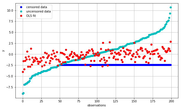
我们可以看到，我们在低于真实值下估计 $y$ ，反之亦然（红色与青色）。这是由于使用了有审查（蓝色）的观察结果，这些观察结果对趋势线产生了很大的影响，将其拉向红色和蓝色点之间的误差。

使用无审查数据的OLS

为了保持分析的可处理性，最简单的方法是简单地忽略所有审查观测结果。

\[\begin{array}{ll} \underset{c}{\mbox{minimize}} & \sum_{i=1}^M (y^{(i)} - c^T x^{(i)})^2 \end{array}\]

考虑到我们的 $M$ 远小于 $K$ ，我们为了做到这一点而扔掉了大多数数据集，让我们看看这个新的回归如何工作。

examples/applications/censored_data_files/censored_data_10_0.png

Now, by incorporating these additional constraints, we can see that the predictions are no longer below $D$ for the censored portion. The overall fit has improved and it properly takes into account the boundaries of the censored data.

```python

import cvxpy as cp X_uncensored = X_ordered[:M, :] c = cp.Variable(shape=n) objective = cp.Minimize(cp.sum_squares(X_uncensored*c - y_ordered[:M])) constraints = [ X_ordered[M:,:]*c >= D] prob = cp.Problem(objective, constraints) result = prob.solve()

c_cvx = np.array(c.value).flatten() fit_cvx = X_ordered.dot(c_cvx) plot_fit(fit_cvx, ‘CVX fit’)

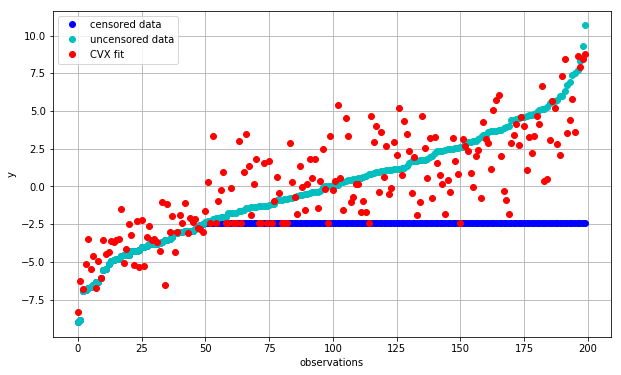
从质量上看，这个拟合结果已经比之前好了，因为它不再对未被审查的部分预测不一致的值。但是它是否能够找到与原始数据接近的系数 $c$ 呢？

我们将使用简单的欧氏距离 $\|c_\mbox{true} - c\|_2$ 来进行比较：

print("norm(c_true - c_cvx): {:.2f}".format(np.linalg.norm((c_true - c_cvx))))
print("norm(c_true - c_ols_uncensored): {:.2f}".format(np.linalg.norm((c_true - c_ols_uncensored))))

norm(c_true - c_cvx): 1.49
norm(c_true - c_ols_uncensored): 2.23

结论 ———-将带有参数分布的被审查数据进行拟合往往是具有挑战性的，因为最大似然估计（MLE）的解往往无法通过解析计算得到。然而，许多MLE问题可以转化为凸优化问题，如上所示。随着易于使用且健壮的数值计算软件包的出现，我们现在可以轻松地解决这些问题，同时在数据的各个部分上强制执行一致性条件，以考虑到我们的全部信息集合。