分析:评估与结果分析
简介
分析 旨在展示 日内交易 的图形报告,帮助用户以可视化方式评估和分析投资组合。以下是可查看的一些图形:
- analysis_position
report_graph
score_ic_graph
cumulative_return_graph
risk_analysis_graph
rank_label_graph
- analysis_model
model_performance_graph
Qlib 中所有累积收益指标(如收益、最大回撤)均通过求和计算,以避免指标或图表随时间呈指数偏斜。
图形报告
用户可以运行以下代码获取所有支持的报告。
>> import qlib.contrib.report as qcr
>> print(qcr.GRAPH_NAME_LIST)
['analysis_position.report_graph', 'analysis_position.score_ic_graph', 'analysis_position.cumulative_return_graph', 'analysis_position.risk_analysis_graph', 'analysis_position.rank_label_graph', 'analysis_model.model_performance_graph']
注意
更多详细信息,请参阅函数文档:类似 help(qcr.analysis_position.report_graph)
用法与示例
analysis_position.report 的用法
API
图形结果
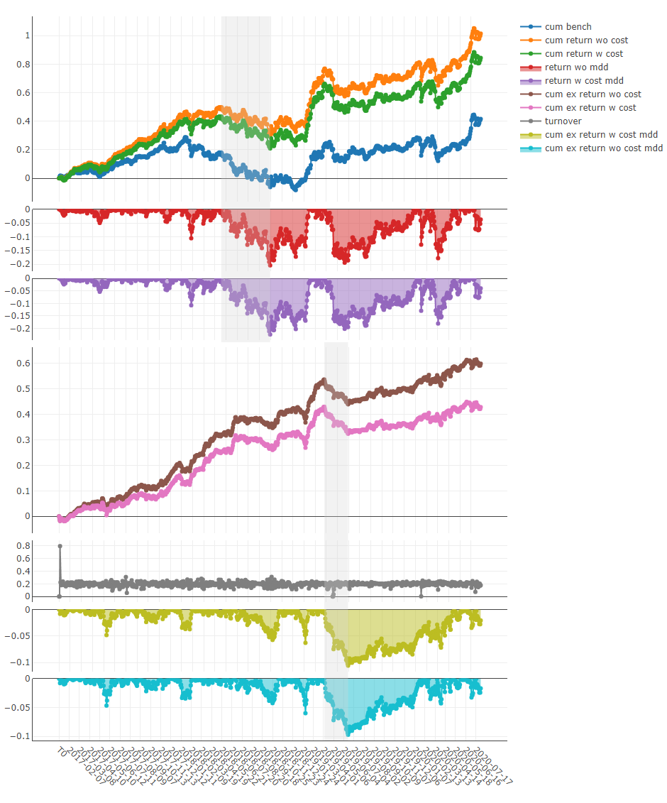
注意
X 轴:交易日
- Y 轴:
- cum bench
基准的累积收益序列
- cum return wo cost
不考虑成本的投资组合累积收益序列
- cum return w cost
考虑成本的投资组合累积收益序列
- return wo mdd
不考虑成本的累积收益最大回撤序列
- return w cost mdd:
考虑成本的累积收益最大回撤序列
- 无成本累积超额收益
投资组合与基准相比的无成本累积异常收益(CAR)序列。
- 有成本累积超额收益
投资组合与基准相比的有成本累积异常收益(CAR)序列。
- 换手率
换手率序列
- 无成本累积超额收益最大回撤
无成本累积异常收益(CAR)的回撤序列
- 有成本累积超额收益最大回撤
有成本累积异常收益(CAR)的回撤序列
上方阴影部分:对应于 无成本累积收益 的最大回撤
下方阴影部分:对应于 无成本累积超额收益 的最大回撤
使用 analysis_position.score_ic
API
图形结果
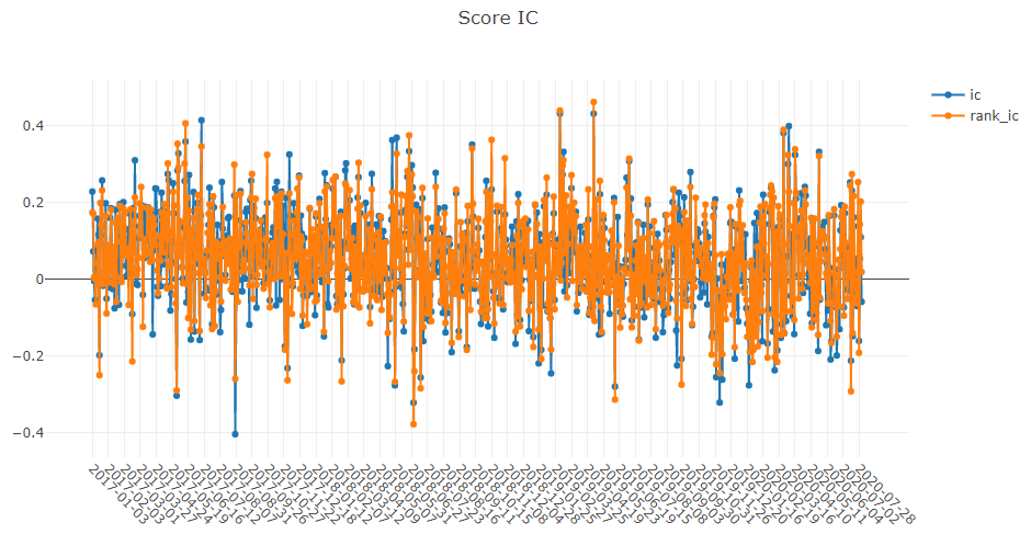
注意
X 轴:交易日
- Y 轴:
- ic
标签 与 预测得分 之间的 皮尔逊相关系数 序列。在上例中,标签 定义为 Ref($close, -2)/Ref($close, -1)-1。更多详情请参阅 数据特征。
- rank_ic
标签 与 预测得分 之间的 斯皮尔曼等级相关系数 序列。
使用 analysis_position.risk_analysis
API
图形结果
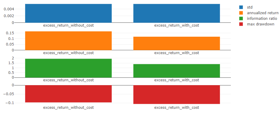
注意
- 通用图表
- std
- 无成本超额收益
无成本累积异常收益(CAR)的 标准差。
- 有成本超额收益
有成本累积异常收益(CAR)的 标准差。
- 年化收益
- 无成本超额收益
无成本累积异常收益(CAR)的 年化收益率。
- 有成本超额收益
有成本累积异常收益(CAR)的 年化收益率。
- 信息比率
- 无成本超额收益
无成本的 信息比率。
- 有成本超额收益
有成本的 信息比率。
欲了解更多关于信息比率的信息,请参阅信息比率 – IR。
- 最大回撤
- 无成本超额收益
不考虑成本的CAR(累计异常收益)的最大回撤。
- 有成本超额收益
考虑成本的CAR(累计异常收益)的最大回撤。
注意
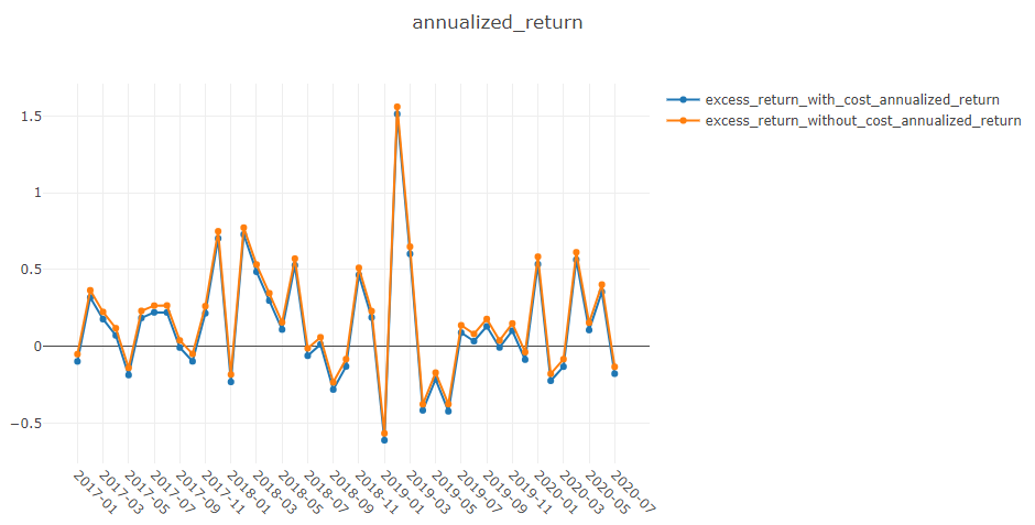
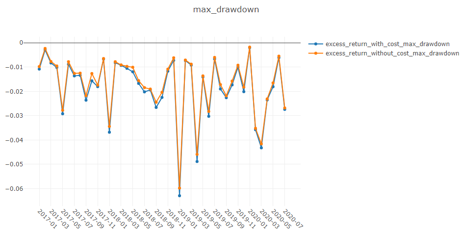
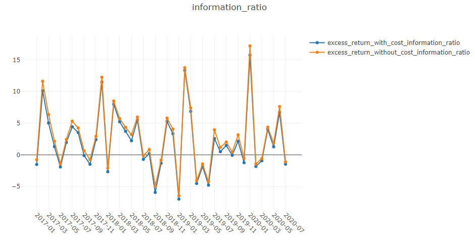
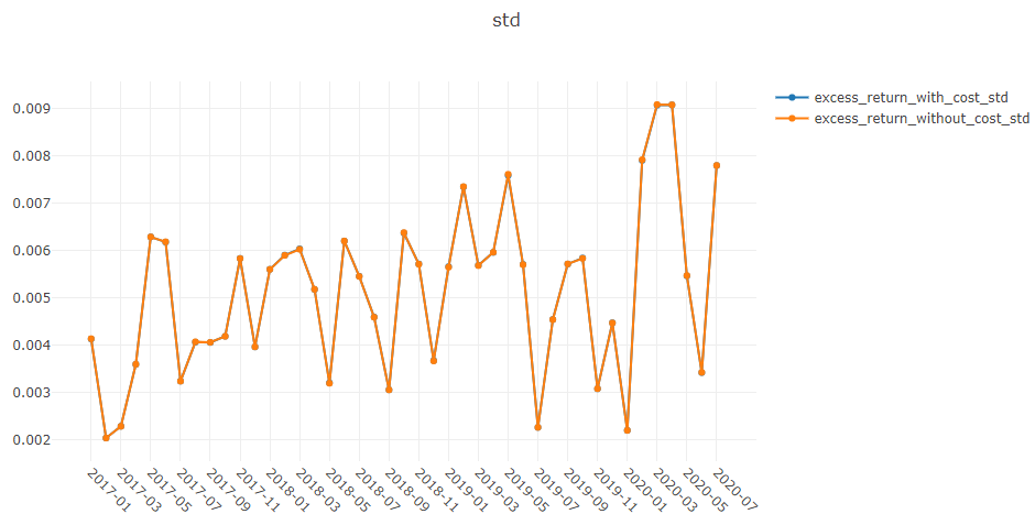
- 年化收益/最大回撤/信息比率/标准差图表
X 轴:按月分组的交易日
- Y 轴:
- 年化收益图表
- 不考虑成本的年化超额收益
不考虑成本的月度CAR(累计异常收益)的年化收益率序列。
- 考虑成本的年化超额收益
考虑成本的月度CAR(累计异常收益)的年化收益率序列。
- 最大回撤图表
- 不考虑成本的最大回撤超额收益
不考虑成本的月度CAR(累计异常收益)的最大回撤序列。
- 考虑成本的最大回撤超额收益
考虑成本的月度CAR(累计异常收益)的最大回撤序列。
- 信息比率图表
- 不考虑成本的信息比率超额收益
不考虑成本的月度CAR(累计异常收益)的信息比率序列。
- 考虑成本的信息比率超额收益
考虑成本的月度CAR(累计异常收益)的信息比率序列。
- 标准差图表
- 不考虑成本的最大回撤超额收益
不考虑成本的月度CAR(累计异常收益)的标准差序列。
- 考虑成本的最大回撤超额收益
考虑成本的月度CAR(累计异常收益)的标准差序列。
使用analysis_model.analysis_model_performance
API
图形结果
注意
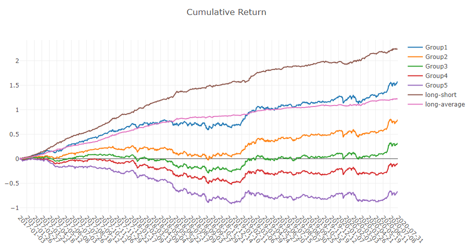
- 累计收益图表
- 组 1:
累计收益序列(标签的排名比例 ≤ 20%的股票组)
- 组 2:
股票组的累计收益系列(20% < 标签的排名比例 ≤ 40%)
- 第 3 组:
股票组的累计收益系列(40% < 标签的排名比例 ≤ 60%)
- 第 4 组:
股票组的累计收益系列(60% < 标签的排名比例 ≤ 80%)
- 第 5 组:
股票组的累计收益系列(80% < 标签的排名比例)
- 多空:
第 1 组与第 5 组的累计收益之间的差值系列
- 多-平均
第 1 组的累计收益与所有股票的平均累计收益之间的差值系列
- 排名比例可表示为如下公式。
- \[排名比例 = \frac{标签的升序排名}{投资组合中的股票数量}\]
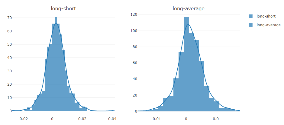
注意
- 多空/多-平均
每个交易日多空/多-平均收益的分布
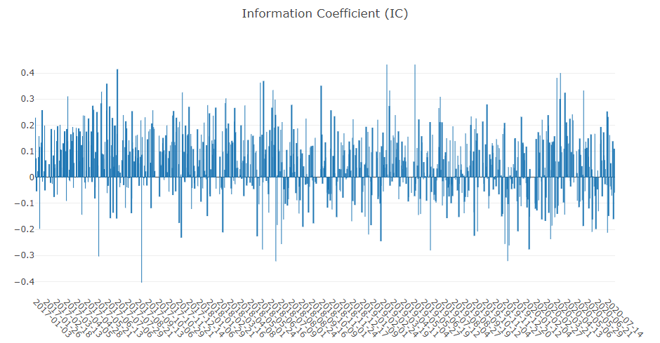
注意
- 信息系数
投资组合中股票的标签与预测得分之间的皮尔逊相关系数系列。
图形报告可用于评估预测得分。
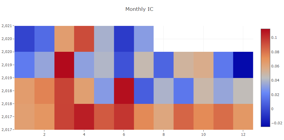
注意
- 月度 IC
信息系数的月度平均值
注意
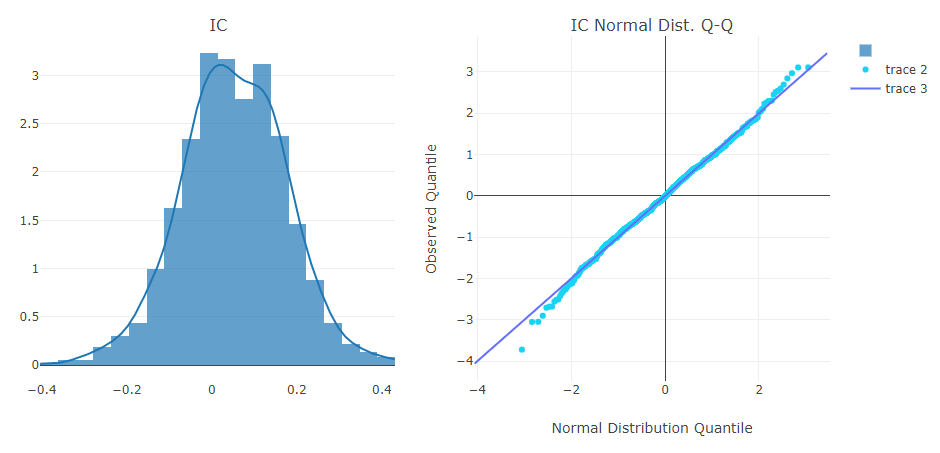
- IC
每个交易日信息系数的分布。
- IC 正态分布 Q-Q 图
分位数-分位数图用于展示每个交易日信息系数的正态分布情况。
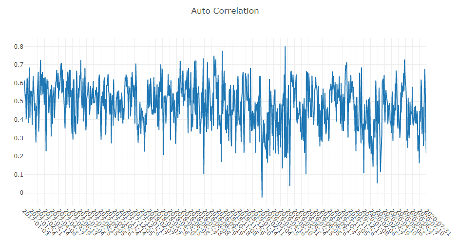
注意
- 自相关
每个交易日投资组合中股票的最新预测得分与lag天前的预测得分之间的皮尔逊相关系数系列。
图形报告可用于估算换手率。